Simplex

From Wikipedia, the free encyclopedia

For other uses, see Simplex (disambiguation).

In geometry, a simplex (plural simplexes or simplices) or n-simplex is an n-dimensional analogue of a triangle. Specifically, a simplex is the convex hull of a set of (n + 1) affinely independent points in some Euclidean space of dimension n or higher (i.e., a set of points such that no m-plane contains more than (m + 1) of them; such points are said to be in general position).

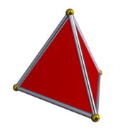
For example, a 0-simplex is a point, a 1-simplex is a line segment, a 2-simplex is a triangle, a 3-simplex is a tetrahedron, and a 4-simplex is a pentachoron (in each case with interior).

A regular simplex is a simplex that is also a regular polytope. A regular n-simplex may be constructed from a regular (n − 1)-simplex by connecting a new vertex to all original vertices by the common edge length.

[edit] Elements

The convex hull of any nonempty subset of the n+1 points that define an n-simplex is called a face of the simplex. Faces are simplices themselves. In particular, the convex hull of a subset of size m+1 (of the n+1 defining points) is an m-simplex, called an m-face of the n-simplex. The 0-faces (i.e., the defining points themselves as sets of size 1) are called the vertices (singular: vertex), the 1-faces are called the edges, the (n − 1)-faces are called the facets, and the sole n-face is the whole n-simplex itself. In general, the number of m-faces is equal to the binomial coefficient C(n + 1, m + 1). Consequently, the number of m-faces of an n-simplex may be found in column (m + 1) of row (n + 1) of Pascal's triangle. A simplex A is a coface of a simplex B if B is a face of A. Face and facet can have different meanings when describing types of simplices in a simplicial complex. See Simplicial_complex#Definitions

The regular simplex family is the first of three regular polytope families, labeled by Coxeter as α_n, the other two being the cross-polytope family, labeled as β_n, and the hypercubes, labeled as γ_n. A fourth family, the infinite tessellation of hypercubes he labeled as δ_n.

n-Simplex elements (sequence A135278 in OEIS)
Δⁿ	α_n	n-polytope	Name	Schläfli symbol Coxeter-Dynkin	Vertices 0-faces	Edges 1-faces	Faces 2-faces	Cells 3-faces	4-faces	5-faces	6-faces	7-faces	8-faces	9-faces
Δ⁰	α₀	0-polytope	Point (0-simplex)	-	1
Δ¹	α₁	1-polytope	Line segment (1-simplex)	{}	2	1
Δ²	α₂	2-polytope	Triangle (2-simplex)	{3}	3	3	1
Δ³	α₃	3-polytope	Tetrahedron (3-simplex)	{3,3}	4	6	4	1
Δ⁴	α₄	4-polytope	Pentachoron (4-simplex)	{3,3,3}	5	10	10	5	1
Δ⁵	α₅	5-polytope	Hexateron Hexa-5-tope (5-simplex)	{3,3,3,3}	6	15	20	15	6	1
Δ⁶	α₆	6-polytope	Heptapeton Hepta-6-tope (6-simplex)	{3,3,3,3,3}	7	21	35	35	21	7	1
Δ⁷	α₇	7-polytope	Octaexon Octa-7-tope (7-simplex)	{3,3,3,3,3,3}	8	28	56	70	56	28	8	1
Δ⁸	α₈	8-polytope	Enneazetton Ennea-8-tope (8-simplex)	{3,3,3,3,3,3,3}	9	36	84	126	126	84	36	9	1
Δ⁹	α₉	9-polytope	Decayotton Deca-9-tope (9-simplex)	{3,3,3,3,3,3,3,3}	10	45	120	210	252	210	120	45	10	1
Δ¹⁰	α₁₀	10-polytope	Hendeca-10-tope (10-simplex)	{3,3,3,3,3,3,3,3,3}	11	55	165	330	462	462	330	165	55	11

In some conventions,^[who?] the empty set is defined to be a (−1)-simplex. The definition of the simplex above still makes sense if n = −1. This convention is more common in applications to algebraic topology (such as simplicial homology) than to the study of polytopes.

[edit] The standard simplex

The standard 2-simplex in R³

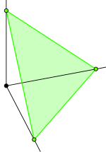
The standard n-simplex (or unit n-simplex) is the subset of Rⁿ⁺¹ given by

$\Delta^n = \left\{(t_0,\cdots,t_n)\in\mathbb{R}^{n+1}\mid\Sigma_{i}{t_i} = 1 \mbox{ and } t_i \ge 0 \mbox{ for all } i\right\}$

The simplex Δⁿ live in the affine hyperplane obtained by removing the restriction t_i ≥ 0 in the above definition. The standard simplex is clearly regular.

The vertices of the standard n-simplex are the points

e₀ = (1, 0, 0, …, 0),

e₁ = (0, 1, 0, …, 0),

$\vdots$

e_n = (0, 0, 0, …, 1).

There is a canonical map from the standard n-simplex to an arbitrary n-simplex with vertices (v₀, …, v_n) given by

$(t_0,\cdots,t_n) \mapsto \Sigma_i t_i v_i$

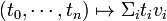
The coefficients t_i are called the barycentric coordinates of a point in the n-simplex. Such a general simplex is often called an affine n-simplex, to emphasize that the canonical map is an affine transformation. It is also sometimes called an oriented affine n-simplex to emphasize that the canonical map may be orientation preserving or reversing.

[edit] Geometric properties

The oriented volume of an n-simplex in n-dimensional space with vertices (v₀, ..., v_n) is

${1\over n!}\det \begin{pmatrix} v_1-v_0 & v_2-v_0& \dots & v_{n-1}-v_0 & v_n-v_0 \end{pmatrix}$

where each column of the n × n determinant is the difference between the vectors representing two vertices. Without the 1/n! it is the formula for the volume of an n-parallelepiped. One way to understand the 1/n! factor is as follows. If the coordinates of a point in a unit n-box are sorted, together with 0 and 1, and successive differences are taken, then since the results add to one, the result is a point in an n simplex spanned by the origin and the closest n vertices of the box. The taking of differences was a unimodular (volume-preserving) transformation, but sorting compressed the space by a factor of n!.

The volume under a standard n-simplex (i.e. between the origin and the simplex in Rⁿ⁺¹) is

${1 \over (n+1)!}$

The volume of a regular n-simplex with unit side length is

${\frac{\sqrt{n+1}}{n!\sqrt{2^n}}}$

as can be seen by multiplying the previous formula by xⁿ⁺¹, to get the volume under the n-simplex as a function of its vertex distance x from the origin, differentiating with respect to x, at $x=1/\sqrt{2}$ (where the n-simplex side length is 1), and normalizing by the length $dx/\sqrt{n+1}\,$ of the increment, $(dx/(n+1),\dots, dx/(n+1))$ , along the normal vector.

[edit] Simplexes with an "orthogonal corner"

Orthogonal corner means here, that there is a vertex at which all adjacent hyperfaces are pairwise orthogonal. Such simplexes are generalizations of right angle triangles and for them there exists a n-dimensional version of the Pythagorean theorem:

The sum of the squared n-dimensional volumes of the hyperfaces adjacent to the orthogonal corner equals the squared n-dimensional volume of the hyperface opposite of the orthogonal corner.

$\sum_{k=1}^{n} |A_{k}|^2 = |A_{0}|^2$

where $A_{1} \ldots A_{n}$ are hyperfaces being pairwise orthogonal to each other but not orthogonal to $A 0$ , which is the hyperface opposite of the orthogonal corner.

For a 2-simplex the theorem is the Pythagorean theorem for triangles with a right angle and for a 3-simplex it is de Gua's theorem for a tetrahedron with a cube corner.

[edit] Relation to the (n+1)-hypercube

The Hasse diagram of the face lattice of an n-simplex is isomorphic to the graph of the (n+1)-hypercube's edges, with the hypercube's vertices mapping to each of the n-simplex's elements, including the entire simplex and the null polytope as the extreme points of the lattice (mapped to two opposite vertices on the hypercube). This fact may be used to efficiently enumerate the simplex's face lattice, since more general face lattice enumeration algorithms are more computationally expensive.

The n-simplex is also the vertex figure of the (n+1)-hypercube.

[edit] Topology

Topologically, an n-simplex is equivalent to an n-ball. Every n-simplex is an n-dimensional manifold with boundary.

[edit] Probability

Main article: Categorical distribution

In probability theory, the points of the standard n-simplex in $(n + 1)$ -space are the space of possible parameters (probabilities) of the categorical distribution on n+1 possible outcomes.

[edit] Algebraic topology

In algebraic topology, simplices are used as building blocks to construct an interesting class of topological spaces called simplicial complexes. These spaces are built from simplices glued together in a combinatorial fashion. Simplicial complexes are used to define a certain kind of homology called simplicial homology.

A finite set of k-simplexes embedded in an open subset of Rⁿ is called an affine k-chain. The simplexes in a chain need not be unique; they may occur with multiplicity. Rather than using standard set notation to denote an affine chain, it is instead the standard practice to use plus signs to separate each member in the set. If some of the simplexes have the opposite orientation, these are prefixed by a minus sign. If some of the simplexes occur in the set more than once, these are prefixed with an integer count. Thus, an affine chain takes the symbolic form of a sum with integer coefficients.

Note that each face of an n-simplex is an affine n-1-simplex, and thus the boundary of an n-simplex is an affine n-1-chain. Thus, if we denote one positively-oriented affine simplex as

σ = [v 0, v 1, v 2,..., v n]

with the $v j$ denoting the vertices, then the boundary $\partial\sigma$ of σ is the chain

$\partial\sigma = \sum_{j=0}^n (-1)^j [v_0,...,v_{j-1},v_{j+1},...,v_n]$ .

More generally, a simplex (and a chain) can be embedded into a manifold by means of smooth, differentiable map 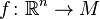$f\colon\mathbb{R}^n\rightarrow M$ . In this case, both the summation convention for denoting the set, and the boundary operation commute with the embedding. That is,

$f(\sum\nolimits_i a_i \sigma_i) = \sum\nolimits_i a_i f(\sigma_i)$

where the $a i$ are the integers denoting orientation and multiplicity. For the boundary operator $\partial$ , one has:

$\partial f(\rho) = f (\partial \rho)$

where ρ is a chain. The boundary operation commutes with the mapping because, in the end, the chain is defined as a set and little more, and the set operation always commutes with the map operation (by definition of a map).

A continuous map $f:\sigma\rightarrow X$ to a topological space X is frequently referred to as a singular n-simplex.

[edit] Random sampling

(Also called Simplex Point Picking) There are at least two efficient ways to generate uniform random samples from the unit simplex.

The first method is based on the fact that sampling from the K-dimensional unit simplex is equivalent to sampling from a Dirichlet distribution with parameters α = (α₁, ..., α_K) all equal to one. The exact procedure would be as follows:

Generate K unit-exponential distributed random draws x₁, ..., x_K.
- This can be done by generating K uniform random draws y_i from the open interval (0,1) and setting x_i=-ln(y_i).
Set S to be the sum of all the x_i.
The K coordinates t₁, ..., t_K of the final point on the unit simplex are given by t_i=x_i/S.

The second method to generate a random point on the unit simplex is based on the order statistics of the uniform distribution on the unit interval (see Devroye, p.568). The algorithm is as follows:

Set p₀ = 0 and p_K=1.
Generate K-1 uniform random draws p_i from the open interval (0,1).
Sort into ascending order the K+1 points p₀, ..., p_K.
The K coordinates t₁, ..., t_K of the final point on the unit simplex are given by t_i=p_i-p_i-1.

[edit] Random walk

Sometimes, rather than picking a point on the simplex at random we need to perform a uniform random walk on the simplex. Such random walks are frequently required for Monte Carlo method computations such as Markov chain Monte Carlo over the simplex domain.

An efficient algorithm to do the walk can be derived from the fact that the normalized sum of K unit-exponential random variables is distributed uniformly over the simplex. We begin by defining a univariate function that "walks" a given sample over the positive real line such that the stationary distribution of its samples is the unit-exponential distribution. The function makes use of the Metropolis-Hastings algorithm to sample the new point given the old point. Such a function can be written as the following, where h is the relative step-size:

next_point <- function(x_old)
{
    repeat {
        x_new <- x_old * exp( Random_Normal(0,h) )
        metropolis_ratio <- exp(-x_new) / exp(-x_old)
        hastings_ratio <- ( x_new / x_old )
        acceptance_probability <- min( 1 , metropolis_ratio * hastings_ratio )
        if ( acceptance_probability > Random_Uniform(0,1) ) break
    }
    return(x_new)
}

Then to perform a random walk over the simplex:

Begin by drawing each element x_i, i= 1, 2, ..., K, from a unit-exponential distribution.
For each i= 1, 2, ..., K
- x_i ← next_point(x_i)
Set S to the sum of all the x_i
Set t_i = x_i/S for all i= 1, 2, ..., K

The set of t_i will be restricted to the simplex, and will walk ergodically over the domain with a uniform stationary density. Note that it is important not to re-normalize the x_i at each step; doing so will result in a non-uniform stationary distribution. Instead, think of the x_i as "hidden" parameters, with the simplex coordinates given by the set of t_i.

This procedure effectively samples x_new from a gamma random variable with mean of x_old and standard deviation of h*x_old. If library routines are available to generate the requisite gamma variate directly, they may be used instead. The Hastings ratio for the MCMC step (which is different and independent of the Hastings-ratio in the next_point function) can then be computed given the gamma density function. Although it is theoretically possible to sample from a gamma density directly, experience shows that doing so is numerically unstable. In contrast, the next_point function is numerically stable even after many, many iterations.

[edit] See also

Causal dynamical triangulation
Distance geometry
Delaunay triangulation
Hill tetrahedron
Other regular n-polytopes
- Hypercube
- Cross-polytope
3-sphere
Tesseract
Polychoron
Polytope
List of regular polytopes
Schläfli orthoscheme
Simplex algorithm - a method for solving optimisation problems with inequalities.
Simplicial complex
Simplicial homology
Simplicial set

[edit] External links

Olshevsky, George, Simplex at Glossary for Hyperspace.
OEIS sequence A135278 Triangle read by rows, giving the numbers T(n,m) = binomial(n+1,m+1); or, Pascal's triangle A007318 with its left-hand edge removed.

[edit] References

Walter Rudin, Principles of Mathematical Analysis (Third Edition), (1976) McGraw-Hill, New York, ISBN 0-07-054235-X (See chapter 10 for a simple review of topological properties.).
Andrew S. Tanenbaum, Computer Networks (4th Ed), (2003) Prentice Hall, ISBN 0-13-066102-3 (See 2.5.3).
Luc Devroye, Non-Uniform Random Variate Generation. (1986) ISBN 0-387-96305-7.
H.S.M. Coxeter, Regular Polytopes, Third edition, (1973), Dover edition, ISBN 0-486-61480-8
- p120-121
- p.296, Table I (iii): Regular Polytopes, three regular polytopes in n-dimensions (n>=5)
Eric W. Weisstein, Simplex at MathWorld.

Simplex

From Wikipedia, the free encyclopedia

Contents

[edit] Elements

[edit] The standard simplex

[edit] Geometric properties

[edit] Simplexes with an "orthogonal corner"

[edit] Relation to the (n+1)-hypercube

[edit] Topology

[edit] Probability

[edit] Algebraic topology

[edit] Random sampling

[edit] Random walk

[edit] See also

[edit] External links

[edit] References

Views

Personal tools

Navigation

Search

Interaction

Toolbox

Languages