Exponential decay

From Wikipedia, the free encyclopedia

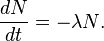
A quantity undergoing exponential decay. Larger decay constants make the quantity vanish much more rapidly. This plot shows decay for decay constants of 25, 5, 1, 1/5, and 1/25 for x from 0 to 4.

A quantity is said to be subject to exponential decay if it decreases at a rate proportional to its value. Symbolically, this can be expressed as the following differential equation, where N is the quantity and λ is a positive number called the decay constant.

$\frac{dN}{dt} = -\lambda N.$

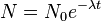
The solution to this equation (see below for derivation) is:

$N(t) = N_0 e^{-\lambda t}. \,$

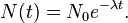
Here N(t) is the quantity at time t, and N₀ = N(0) is the initial quantity, i.e. the quantity at time t = 0.

[edit] Measuring rates of decay

[edit] Mean lifetime

If the decaying quantity is the number of discrete elements of a set, it is possible to compute the average length of time for which an element remains in the set. This is called the mean lifetime (or simply the lifetime) and it can be shown that it relates to the decay rate,

$\tau = \frac{1}{\lambda}.$

The mean lifetime (also called the exponential time constant) is thus seen to be a simple "scaling time":

$N(t) = N_0 e^{-t/\tau}. \,$

Thus, it is the time needed for the assembly to be reduced by a factor of e.

A very similar equation will be seen below, which arises when the base of the exponential is chosen to be 2, rather than e. In that case the scaling time is the "half-life".

[edit] Half-life

Main article: Half-life

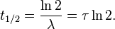
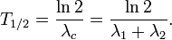
A more intuitive characteristic of exponential decay for many people is the time required for the decaying quantity to fall to one half of its initial value. This time is called the half-life, and often denoted by the symbol $t 1 / 2$ . The half-life can be written in terms of the decay constant, or the mean lifetime, as:

$t_{1/2} = \frac{\ln 2}{\lambda} = \tau \ln 2.$

When this expression is inserted for $τ$ in the exponential equation above, and ln2 is absorbed into the base, this equation becomes:

$N(t) = N_0 2^{-t/t_{1/2}}. \,$

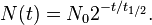
Thus, the amount of material left is $2 - 1 = 1 / 2$ raised to the (whole or fractional) number of half-lives that have passed. Thus, after 3 half-lives there will be $1 / 2 3 = 1 / 8$ of the original material left.

Therefore, the mean lifetime $τ$ is equal to the half-life divided by the natural log of 2, or:

$\tau = \frac{t_{1/2}}{ln 2} = t_{1/2}*1.442695040888963$ .

E.g. Polonium-210 has a half-life of 138 days, and a mean lifetime of 200 days.

[edit] Solution of the differential equation

The equation that describes exponential decay is

$\frac{dN(t)}{dt} = -\lambda N(t)$

or, by rearranging,

$\frac{dN(t)}{N(t)} = -\lambda dt.$

Integrating, we have

$\ln N(t) = -\lambda t + C \,$

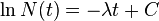
where C is the constant of integration, and hence

$N(t) = e^C e^{-\lambda t} = N_0 e^{-\lambda t} \,$

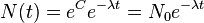
where the final substitution, $N 0 = e C$ , is obtained by evaluating the equation at $t = 0$ , as $N 0$ is defined as being the quantity at $t = 0$ .

This is the form of the equation that is most commonly used to describe exponential decay. Any one of decay constant, mean lifetime or half-life is sufficient to characterise the decay. The notation λ for the decay constant is a remnant of the usual notation for an eigenvalue. In this case, λ is the eigenvalue of the opposite of the differentiation operator with $N (t)$ as the corresponding eigenfunction. The units of the decay constant are s^-1.

[edit] Derivation of the mean lifetime

Given an assembly of elements, the number of which decreases ultimately to zero, the mean lifetime, $τ$ , (also called simply the lifetime) is the expected value of the amount of time before an object is removed from the assembly. Specifically, if the individual lifetime of an element of the assembly is the time elapsed between some reference time and the removal of that element from the assembly, the mean lifetime is the arithmetic mean of the individual lifetimes.

Starting from the population formula

$N = N_0 e^{-\lambda t} \,$ ,

we firstly let c be the normalizing factor to convert to a probability space:

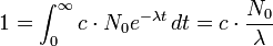
$1 = \int_{0}^{\infty}c \cdot N_0 e^{-\lambda t}\, dt = c \cdot \frac{N_0}{\lambda}$

or, on rearranging,

$c = \frac{\lambda}{N_0}.$

We see that exponential decay is a scalar multiple of the exponential distribution (i.e. the individual lifetime of a each object is exponentially distributed), which has a well-known expected value. We can compute it here using integration by parts.

$\tau = \langle t \rangle = \int_{0}^{\infty} t \cdot c \cdot N_0 e^{-\lambda t}\, dt = \int_{0}^{\infty} \lambda t e^{-\lambda t}\, dt = \frac{1}{\lambda}.$

[edit] Decay by two or more processes

A quantity may decay via two or more different processes simultaneously. In general, these processes (often called "decay modes", "decay channels", "decay routes" etc.) have different probabilities of occurring, and thus occur at different rates with different half-lives, in parallel. The total decay rate of the quantity N is given by the sum of the decay routes; thus, in the case of two processes:

$-\frac{dN(t)}{dt} = N\lambda _1 + N\lambda _2 = (\lambda _1 + \lambda _2)N.\,$

The solution to this equation is given in the previous section, where the sum of $\lambda _1 + \lambda _2\,$ is treated as a new total decay constant $\lambda _c\,$ .

$N(t) = N_0 e^{-(\lambda _1 + \lambda _2) t} = N_0 e^{-(\lambda _c) t}.\,$

Since $\tau = 1/\lambda\,$ , a combined $\tau_c\,$ can be given in terms of $\lambda\,$ s:

$\frac{1}{\tau_c} = \lambda_c = \lambda_1 + \lambda_2 = \frac{1}{\tau_1} + \frac{1}{\tau_2}\,$

$\tau_c = \frac{\tau_1 \tau_2}{\tau_1 + \tau_2}.\,$

In words: the mean life for combined decay channels is the harmonic mean of the mean lives associated with the individual processes divided by the total number of processes.

Since half-lives differ from mean life $\tau\,$ by a constant factor, the same equation holds in terms of the two corresponding half-lives:

$T_{1/2} = \frac{t_1 t_2}{t_1 + t_2} \,$

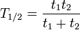
where $T 1 / 2$ is the combined or total half-life for the process, $t 1$ is the half-life of the first process, and $t 2$ is the half life of the second process.

In terms of separate decay constants, the total half-life $T 1 / 2$ can be shown to be

$T_{1/2} = \frac{\ln 2}{\lambda _c} = \frac{\ln 2}{\lambda _1 + \lambda _2}.\,$

For a decay by three simultaneous exponential processes the total half-life can be computed, as above, as the harmonic mean of separate mean lives:

$T_{1/2} = \frac{t_1 t_2 t_3}{(t_1 t_2) + (t_1 t_3) + (t_2 t_3)} = \frac{\ln 2}{\lambda _c} = \frac{\ln 2}{\lambda_1 + \lambda_2 + \lambda_3}.\,$

[edit] Applications and examples

Exponential decay occurs in a wide variety of situations. Most of these fall into the domain of the natural sciences. Any application of mathematics to the social sciences or humanities is risky and uncertain, because of the extraordinary complexity of human behavior. However, a few roughly exponential phenomena have been identified there as well.

Many decay processes that are often treated as exponential, are really only exponential so long as the sample is large and the law of large numbers holds. For small samples, a more general analysis is necessary, accounting for a Poisson process.

[edit] Natural sciences

In a sample of a radionuclide that undergoes radioactive decay to a different state, the number of atoms in the original state follows exponential decay as long as the remaining number of atoms is large. The decay product is termed a radiogenic nuclide.

If an object at one temperature is exposed to a medium of another temperature, the temperature difference between the object and the medium follows exponential decay (in the limit of slow processes; equivalent to "good" heat conduction inside the object, so that its temperature remains relatively uniform through its volume). See also Newton's law of cooling.

The rates of certain types of chemical reactions depend on the concentration of one or another reactant. Reactions whose rate depends only on the concentration of one reactant (known as first-order reactions) consequently follow exponential decay. For instance, many enzyme-catalyzed reactions behave this way.

Atmospheric pressure decreases approximately exponentially with increasing height above sea level, at a rate of about 12% per 1000m.

The electric charge (or, equivalently, the potential) stored on a capacitor (capacitance C) decays exponentially, if the capacitor experiences a constant external load (resistance R). The exponential time-constant τ for the process is R C, and the half-life is therefore R C ln2. (Furthermore, the particular case of a capacitor discharging through several parallel resistors makes an interesting example of multiple decay processes, with each resistor representing a separate process. In fact, the expression for the equivalent resistance of two resistors in parallel mirrors the equation for the half-life with two decay processes.)

Some vibrations may decay exponentially; this characteristic is often used in creating ADSR envelopes in synthesizers.

In pharmacology and toxicology, it is found that many administered substances are distributed and metabolized (see clearance) according to exponential decay patterns. The biological half-lives "alpha half-life" and "beta half-life" of a substance measure how quickly a substance is distributed and eliminated.

The intensity of electromagnetic radiation such as light or X-rays or gamma rays in an absorbent medium, follows an exponential decrease with distance into the absorbing medium.

The decline in resistance of a Negative Temperature Coefficient Thermistor as temperature is increased.

[edit] Social sciences

The field of glottochronology attempts to determine the time elapsed since the divergence of two languages from a common root, using the assumption that linguistic changes are introduced at a steady rate; given this assumption, we expect the similarity between them (the number of properties of the language that are still identical) to decrease exponentially.

In history of science, some believe that the body of knowledge of any particular science is gradually disproved according to an exponential decay pattern (see half-life of knowledge).

[edit] Computer science

BGP, the core routing protocol on the Internet, has to maintain a routing table in order to remember the paths a packet can be deviated to. When one of this paths repeatedly changes its state from available to not available (and vice-versa), the BGP router controlling that path has to repeatedly add and remove the path record from its routing table (flaps the path), thus spending local resources such as CPU and RAM and, even more, broadcasting unuseful information to peer routers. To prevent this undesired behavior, an algorithm named route flapping damping assigns each route a weight that gets bigger each time the route changes its state and decays exponentially with time. When the weight reaches a certain limit, no more flapping is done, thus suppressing the route.

[edit] See also

Exponential growth

[edit] External links

Exponential decay

From Wikipedia, the free encyclopedia

Contents

[edit] Measuring rates of decay

[edit] Mean lifetime

[edit] Half-life

[edit] Solution of the differential equation

[edit] Derivation of the mean lifetime

[edit] Decay by two or more processes

[edit] Applications and examples

[edit] Natural sciences

[edit] Social sciences

[edit] Computer science

[edit] See also

[edit] External links

Views

Personal tools

Navigation

Search

Interaction

Toolbox

Languages