Spin (physics)

From Wikipedia, the free encyclopedia

This article is about spin in quantum mechanics. For rotation in classical mechanics, see angular momentum. For other uses, see spin (disambiguation).

In quantum mechanics, spin is a fundamental property of atomic nuclei, hadrons, and elementary particles. For particles with non-zero spin, spin direction (also called spin for short) is an important intrinsic degree of freedom.

As the name indicates, the spin has originally been thought of as a rotation of particles around their own axis. This picture is correct insofar as spins obey the same mathematical laws as do quantized angular momenta. On the other hand, spins have some peculiar properties that distinguish them from orbital angular momenta: spins may have half-integer quantum numbers, and the spin of charged particles is associated with a magnetic dipole moment in a way (g-factor different from 1) that is incompatible with classical physics.

Spins have important theoretical implications and practical applications. The electron spin is the key to the Pauli exclusion principle and to the understanding of the periodic system of chemical elements. Spin-orbit coupling leads to the fine structure of atomic spectra, which is used in atomic clocks and in the modern definition of the fundamental unit second. Precise measurements of the g-factor of the electron have played an important role in the development and verification of quantum electrodynamics. Electron spins play an important role in magnetism, with applications for instance in computer memories. Manipulation of spins in semiconductor devices is the subject of the developing field of spintronics. The manipulation of nuclear spins by radiofrequency waves (nuclear magnetic resonance) is important in chemical spectroscopy and medical imaging. The photon spin is associated with the polarization of light.

The concept of a spin, though not the name, was proposed by Wolfgang Pauli in 1924. In 1925, Ralph Kronig, George Uhlenbeck, and Samuel Goudsmit suggested a physical interpretation of particles spinning around their own axis. The mathematical theory was worked out in depth by Pauli in 1927. In 1928, Paul Dirac showed that the electron spin arises naturally within relativistic quantum mechanics.

The head-on collision of a quark (red ball) from one proton (orange ball) with a gluon (green ball) from another proton with opposite spin, spin is represented by the blue arrows circling the protons and the quark. The blue question marks circling the gluon represent the question: Are gluons polarized? Ejected from the collision are a shower of quarks and a photon of light (purple ball).

[edit] The spin quantum number

[edit] Spin of elementary particles

Elementary particles, such as the photon, the electron, and the various quarks are particles that cannot be divided into smaller units. Theoretical and experimental studies have shown that the spin possessed by these particles cannot be explained by postulating that they are made up of even smaller particles rotating about a common center of mass (see classical electron radius); as far as can be determined, these elementary particles are true point particles. The spin that they carry is a truly intrinsic physical property, akin to a particle's electric charge and mass.

In quantum mechanics, the angular momentum of any system is quantized: its magnitude can only take values

$S = \hbar \, \sqrt{s (s+1)},$

where $\hbar$ is the reduced Planck's constant, and the spin quantum number s is a non-negative integer or half-integer (0, 1/2, 1, 3/2, 2, etc.). The possibility of half-integer quantum numbers is a major difference between spin and orbital angular momentum; the latter can only take integer quantum numbers. The value of s depends only on the type of particle, and cannot be altered in any known way (in contrast to the spin direction, see below).

For instance, all electrons have s = 1/2. Other elementary spin-1/2 particles include positrons, neutrinos and quarks. Photons are spin-1 particles, and the hypothetical graviton is a spin-2 particle. The hypothetical Higgs boson is unique among elementary particles in having a spin of zero.

[edit] Spin of composite particles

The spin of composite particles, such as protons, neutrons, and atomic nuclei is usually understood to mean the total angular momentum, which is the sum of the spins and orbital angular momenta of the constituent particles. Such a composite spin is subject to the same quantization condition as any other angular momentum.

Composite particles are often referred to as having a definite spin, just like elementary particles; for example, the proton is a spin-1/2 particle. This is understood to refer to the spin of the lowest-energy internal state of the composite particle (i.e., a given spin and orbital configuration of the constituents).

It is not always easy to deduce the spin of a composite particle from first principles; for example, even though we know that the proton is a spin-1/2 particle, the question of how this spin is distributed among the three internal valence quarks and the surrounding sea quarks and gluons is an active area of research.

[edit] Spin of atoms and molecules

The spin of atoms and molecules is the sum of the spin of unpaired electrons. It is responsible for paramagnetism.

[edit] The spin-statistics connection

The spin of a particle has crucial consequences for its properties in statistical mechanics. Particles with half-integer spin obey Fermi-Dirac statistics, and are known as fermions. They are required to occupy antisymmetric quantum states (see the article on identical particles.) This property forbids fermions from sharing quantum states – a restriction known as the Pauli exclusion principle. Particles with integer spin, on the other hand, obey Bose-Einstein statistics, and are known as bosons. These particles occupy "symmetric states", and can therefore share quantum states. The proof of this is known as the spin-statistics theorem, which relies on both quantum mechanics and the theory of special relativity. In fact, the connection between spin and statistics is one of the most important and remarkable consequences of special relativity.

[edit] Magnetic moments

Particles with spin can possess a magnetic dipole moment, just like a rotating electrically charged body in classical electrodynamics. These magnetic moments can be experimentally observed in several ways, e.g. by the deflection of particles by inhomogeneous magnetic fields in a Stern–Gerlach experiment, or by measuring the magnetic fields generated by the particles themselves.

The intrinsic magnetic moment μ of an elementary particle with charge q, mass m, and spin S, is

$\mu = g \, \frac{q}{2m}\, S$

where the dimensionless quantity g is called the g-factor. For exclusively orbital rotations it would be 1.

The electron, being a charged elementary particle, possesses a nonzero magnetic moment. One of the triumphs of the theory of quantum electrodynamics is its accurate prediction of the electron g-factor, which has been experimentally determined to have the value −2.002 319 304 3622(15), with the digits in parentheses denoting measurement uncertainty in the last two digits at one standard deviation.^[1] The value of 2 arises from the Dirac equation, a fundamental equation connecting the electron's spin with its electromagnetic properties, and the correction of 0.002 319 304… arises from the electron's interaction with the surrounding electromagnetic field, including its own field.^[2] Composite particles also possess magnetic moments associated with their spin. In particular, the neutron possesses a non-zero magnetic moment despite being electrically neutral. This fact was an early indication that the neutron is not an elementary particle. In fact, it is made up of quarks, which are electrically charged particles. The magnetic moment of the neutron comes from the spins of the individual quarks and their orbital motions.

The neutrinos are both elementary and electrically neutral. The minimally extended Standard Model that takes into account finite neutrino masses, predicts neutrino magnetic moments of:^[3]^[4]^[5]

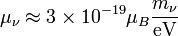
$\mu_{\nu}\approx 3\times 10^{-19}\mu_{B}\frac{m_{\nu}}{\text{eV}}$

where the $μ ν$ are the neutrino magnetic moments, $m ν$ are the neutrino masses, and $μ B$ is the Bohr magneton. New physics above the electroweak scale could, however, lead to significantly higher neutrino magnetic moments. It can be shown in a model independent way that neutrino magnetic moments larger than about 10⁻¹⁴ $μ B$ are unnatural, because they would also lead to large radiative contributions to the neutrino mass. Since the neutrino masses cannot exceed about 1 eV, these radiative corrections must then be assumed to be fine tuned to cancel out to a large degree.^[6]

The measurement of neutrino magnetic moments is an active area of research. As of 2001^[update], the latest experimental results have put the neutrino magnetic moment at less than 1.2 × 10^-10 times the electron's magnetic moment.

In ordinary materials, the magnetic dipole moments of individual atoms produce magnetic fields that cancel one another, because each dipole points in a random direction. Ferromagnetic materials below their Curie temperature, however, exhibit magnetic domains in which the atomic dipole moments are locally aligned, producing a macroscopic, non-zero magnetic field from the domain. These are the ordinary "magnets" with which we are all familiar.

The study of the behavior of such "spin models" is a thriving area of research in condensed matter physics. For instance, the Ising model describes spins (dipoles) that have only two possible states, up and down, whereas in the Heisenberg model the spin vector is allowed to point in any direction. These models have many interesting properties, which have led to interesting results in the theory of phase transitions.

[edit] Spin direction

[edit] Spin projection quantum number and spin multiplicity

In classical mechanics, the angular momentum of a particle possesses not only a magnitude (how fast the body is rotating), but also a direction (the axis of rotation of the particle). Quantum mechanical spin also contains information about direction, but in a more subtle form. Quantum mechanics states that the component of angular momentum measured along any direction (say along the z-axis) can only take on the values

$\hbar s_z, \qquad s_z = - s, - s + 1, \cdots, s - 1, s$

where s is the principal spin quantum number discussed in the previous section. One can see that there are 2s+1 possible values of s_z. The number 2s+1 is called the multiplicity of the spin system. For example, there are only two possible values for a spin-1/2 particle: s_z = +1/2 and s_z = -1/2. These correspond to quantum states in which the spin is pointing in the +z or -z directions respectively, and are often referred to as "spin up" and "spin down". See spin-1/2.

[edit] Spin vector

For a given quantum state, it is possible to describe a spin vector $\lang S \rang$ whose components are the expectation values of the spin components along each axis, i.e., $\lang S \rang = [\lang s_x \rang, \lang s_y \rang, \lang s_z \rang]$ . This vector describes the "direction" in which the spin is pointing, corresponding to the classical concept of the axis of rotation. It turns out that the spin vector is not very useful in actual quantum mechanical calculations, because it cannot be measured directly — s_x, s_y and s_z cannot possess simultaneous definite values, because of a quantum uncertainty relation between them. However, for statistically large collections of particles that have been placed in the same pure quantum state, such as through the use of a Stern-Gerlach apparatus, the spin vector does have a well-defined experimental meaning: It specifies the direction in ordinary space in which a subsequent detector must be oriented in order to achieve the maximum possible probability (100%) of detecting every particle in the collection. For spin-1/2 particles, this maximum probability drops off smoothly as the angle between the spin vector and the detector increases, until at an angle of 180 degrees — that is, for detectors oriented in the opposite direction to the spin vector—the expectation of detecting particles from the collection reaches a minimum of 0%.

As a qualitative concept, the spin vector is often handy because it is easy to picture classically. For instance, quantum mechanical spin can exhibit phenomena analogous to classical gyroscopic effects. For example, one can exert a kind of "torque" on an electron by putting it in a magnetic field (the field acts upon the electron's intrinsic magnetic dipole moment — see the following section). The result is that the spin vector undergoes precession, just like a classical gyroscope.

Mathematically, quantum mechanical spin is not described by a vector as in classical angular momentum. It is described using a family of objects known as spinors. There are subtle differences between the behavior of spinors and vectors under coordinate rotations. For example, rotating a spin-1/2 particle by 360 degrees does not bring it back to the same quantum state, but to the state with the opposite quantum phase; this is detectable, in principle, with interference experiments. To return the particle to its exact original state, one needs a 720 degree rotation. A spin zero particle can only have a single quantum state, even after torque is applied. Rotating a spin-2 particle 180 degree can bring it back to the same quantum state and a spin-4 particle should be rotated 90 degrees to bring it back to the same quantum state. The spin 2 particle can be analogous to a straight stick that looks the same even after it is rotated 180 degrees and a spin 0 particle can be imagined as sphere which looks the same after whatever angle it is turned through.

[edit] Mathematical formulation of spin in quantum mechanics

[edit] Spin operator

Spin obeys commutation relations analogous to those of the orbital angular momentum:

$[S_i, S_j ] = i \hbar \epsilon_{ijk} S_k$

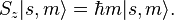
where $ε i j k$ is the Levi-Civita symbol. It follows (as with angular momentum) that the eigenvectors of $S 2$ and $S z$ (expressed as kets in the total $S$ basis) are:

$S^2 |s,m\rangle = \hbar^2 s(s + 1) |s,m\rangle$

$S_z |s,m\rangle = \hbar m |s,m\rangle.$

The spin raising and lowering operators acting on these eigenvectors give:

$S_\pm |s,m\rangle = \hbar\sqrt{s(s+1)-m(m\pm 1)} |s,m\pm 1 \rangle$ , where $S_\pm = S_x \pm i S_y.$

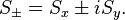
But unlike orbital angular momentum the eigenvectors are not spherical harmonics. They are not functions of $θ$ and $φ$ . There is also no reason to exclude half integer values of s and m.

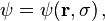In addition to their other properties, all quantum mechanical particles possess an intrinsic spin (though it may have the intrinsic spin 0, too). The spin is quantized in units of the reduced action constant, such that the state function of the particle is, e.g., not $\psi = \psi(\mathbf r)$ , but $\psi =\psi(\mathbf r,\sigma)\,,$ where $σ$ is out of the following discrete set of values:

$\sigma \in \{-s\cdot\hbar , -(s-1)\cdot\hbar , ... ,+(s-1)\cdot\hbar ,+s\cdot\hbar\}$ .

One distinguishes bosons (s=0 or 1 or 2 or ...) and fermions (s=1/2 or 3/2 or 5/2 or ...). The total angular momentum conserved in interaction processes is then the sum of the orbital angular momentum and the spin.

[edit] Spin and the Pauli exclusion principle

For systems of N identical particles this is related to the Pauli exclusion principle, which states that by interchanges of any two of the N particles one must have

$\psi ( \,...\, ;\,\mathbf r_i,\sigma_i\,;\, ...\,;\mathbf r_j,\sigma_j\,;\,...) \stackrel{!}{=}(-1)^{2s}\cdot \psi ( \,...\, ;\,\mathbf r_j,\sigma_j\,;\, ...\,;\mathbf r_i,\sigma_i\,;\,...)\,.$

Thus, for bosons the prefactor $( - 1) 2 s$ will reduce to +1, for fermions to –1. In quantum mechanics all particles are either bosons or fermions. In relativistic quantum field theories also "supersymmetric" particles exist, where linear combinations of bosonic and fermionic components appear. In two dimensions the prefactor $( - 1) 2 s$ can be replaced by any complex number of magnitude 1 (see Anyon).

Electrons are fermions with s=1/2; quanta of light ("photons") are bosons with s=1. This shows also explicitly that the property spin cannot be fully explained as a classical intrinsic orbital angular momentum, e.g., similar to that of a "spinning top", since orbital angular rotations would lead to integer values of s. Instead one is dealing with an essential legacy of relativity. The photon, in contrast, is always relativistic (velocity $v\equiv c)$ , and the corresponding classical theory, that of Maxwell, is also relativistic.

The above permutation postulate for N-particle state functions has most-important consequences in daily life, e.g. the periodic table of the chemists or biologists.

[edit] Spin and rotations

As described above, quantum mechanics states that component of angular momentum measured along any direction can only take a number of discrete values. The most convenient quantum mechanical description of particle's spin is therefore with a set of complex numbers corresponding to amplitudes of finding a given value of projection of its intrinsic angular momentum on a given axis. For instance, for a spin 1/2 particle, we would need two numbers $a_{\pm 1/2}$ , giving amplitudes of finding it with projection of angular momentum equal to $\hbar/2$ and $-\hbar/2$ , satisfying the requirement

$|a_{1/2}|^2 + |a_{-1/2}|^2 \, = 1.$

Since these numbers depend on the choice of the axis, they transform into each other non-trivially when this axis is rotated. It's clear that the transformation law must be linear, so we can represent it by associating a matrix with each rotation, and the product of two transformation matrices corresponding to rotations A and B must be equal (up to phase) to the matrix representing rotation AB. Further, rotations preserve quantum mechanical inner product, and so should our transformation matrices:

$\sum_{m=-j}^{j} a_m^* b_m = \sum_{m=-j}^{j} (\sum_{n=-j}^j U_{nm} a_n)^* (\sum_{k=-j}^j U_{km} b_k)$

$\sum_{n=-j}^j \sum_{k=-j}^j U_{np}^* U_{kq} = \delta_{pq}.$

Mathematically speaking, these matrices furnish a unitary projective representation of the rotation group SO(3). Each such representation corresponds to a representation of the covering group of SO(3), which is SU(2). There is one n-dimensional irreducible representation of SU(2) for each dimension, though this representation is n-dimensional real for odd n and n-dimensional complex for even n (hence of real dimension 2n). For example, spin 1/2 particles transform under rotations according to a 2-dimensional representation, which is generated by Pauli matrices:

$\begin{pmatrix} a_{1/2}' \\ a_{-1/2}' \end{pmatrix} = \exp{(i \sigma_z \gamma / 2)} \exp{(i \sigma_y \beta / 2)} \exp{(i \sigma_x \alpha / 2)} \begin{pmatrix} a_{1/2} \\ a_{-1/2} \end{pmatrix}$

where $α,β,γ$ are Euler angles.

Particles with higher spin transform in a similar way using higher-dimensional representations; see the article on Pauli matrices for matrices generating rotations for spin 1 and 3/2.

[edit] Spin and Lorentz transformations

We could try the same approach to determine the behavior of spin under general Lorentz transformations, but we'd immediately discover a major obstacle. Unlike SO(3), the group of Lorentz transformations SO(3,1) is non-compact and therefore does not have any faithful unitary finite-dimensional representations.

In case of spin 1/2 particles, it is possible to find a construction that includes both a finite-dimensional representation and a scalar product that is preserved by this representation. We associate a 4-component Dirac spinor $ψ$ with each particle. These spinors transform under Lorentz transformations according to the law

$\psi' = \exp{\left(\frac{1}{8} \omega_{\mu\nu} [\gamma_{\mu}, \gamma_{\nu}]\right)} \psi$

where $γ μ$ are gamma matrices and $ω μν$ is an antisymmetric 4x4 matrix parametrizing the transformation. It can be shown that the scalar product

$\langle\psi|\phi\rangle = \bar{\psi}\phi = \psi^{\dagger}\gamma_0\phi$

is preserved. (It is not, however, positive definite, so the representation is not unitary.)

[edit] Pauli matrices and spin operators

The quantum mechanical operators associated with spin observables are:

$S_x = {\hbar \over 2} \sigma_x$

$S_y = {\hbar \over 2} \sigma_y$

$S_z = {\hbar \over 2} \sigma_z$

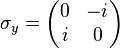
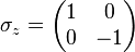
In the special case of spin-1/2 $σ x$ , $σ y$ and $σ z$ are the three Pauli matrices, given by:

$\sigma_x = \begin{pmatrix} 0&1\\ 1&0 \end{pmatrix}$

$\sigma_y = \begin{pmatrix} 0&-i\\ i&0 \end{pmatrix}$

$\sigma_z = \begin{pmatrix} 1&0\\ 0&-1 \end{pmatrix}$

[edit] Measurement of the spin along the x, y, and z axes

Each of the (hermitian) Pauli matrices has two eigenvalues, +1 and -1. The corresponding normalized eigenvectors are:

$\psi_{x+} = \frac{1}{\sqrt{2}} \begin{pmatrix} {1}\\{1}\end{pmatrix}, \psi_{x-} = \frac{1}{\sqrt{2}} \begin{pmatrix} {1}\\{-1}\end{pmatrix}$ ,

$\psi_{y+} = \frac{1}{\sqrt{2}} \begin{pmatrix} {1}\\{i}\end{pmatrix}, \psi_{y-} = \frac{1}{\sqrt{2}} \begin{pmatrix} {1}\\{-i}\end{pmatrix}$ ,

$\psi_{z+} = \begin{pmatrix} 1\\0\end{pmatrix}, \psi_{z-} = \begin{pmatrix} 0\\1\end{pmatrix}$ .

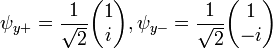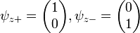By the postulates of quantum mechanics, an experiment designed to measure the electron spin on the x, y or z axis can only yield an eigenvalue of the spin operator ( $S x$ , $S y$ , $S z$ ) on that axis, ${\hbar \over 2}$ and ${-\hbar \over 2}$ . The quantum state of a particle (with respect to spin), can be represented by a two component spinor:

$\psi = \begin{pmatrix} {a+bi}\\{c+di}\end{pmatrix}$

When the spin of this particle is measured with respect to a given axis (in this example, the x-axis), the probability that its spin will be measured as ${\hbar \over 2}$ is just $\mid \langle \psi \mid \psi_{x+} \rangle \mid ^2$ . Correspondingly, the probability that its spin will be measured as ${-\hbar \over 2}$ is just $\mid \langle \psi \mid \psi_{x-} \rangle \mid ^2$ . Following the measurement, the spin state of the particle will collapse into the corresponding eigenstate. As a result, if the particle's spin along a given axis has been measured to have a given eigenvalue, all measurements will yield the same eigenvalue (since $\mid \langle \psi_{x+} \mid \psi_{x+} \rangle \mid ^2 = 1$ , etc), provided that no measurements of the spin are made along other axes (see compatibility section below).

[edit] Measurement of the spin along an arbitrary axis

The operator to measure spin along an arbitrary axis direction is easily obtained from the Pauli spin matrices. Let $u = (u x, u y, u z)$ be an arbitrary unit vector. Then the operator for spin in this direction is simply $S_u = \hbar(u_x\sigma_x + u_y\sigma_y + u_z\sigma_z)/2$ . The operator $S u$ has eigenvalues of $\pm\hbar/2$ , just like the usual spin matrices. This method of finding the operator for spin in an arbitrary direction generalizes to higher spin states, one takes the dot product of the direction with a vector of the three operators for the three x,y,z axis directions.

A normalized spinor for spin-1/2 in the $(u x, u y, u z)$ direction (which works for all spin states except spin down where it will give 0/0), is:

$\frac{1}{\sqrt{2+2u_z}}\begin{bmatrix} 1+u_z \\ u_x+iu_y \end{bmatrix}.$

The above spinor is obtained in the usual way by diagonalizing the $σ u$ matrix and finding the eigenstates corresponding to the eigenvalues.

[edit] Compatibility of spin measurements

Since the Pauli matrices do not commute, measurements of spin along the different axes are incompatible. This means that if, for example, we know the spin along the x-axis, and we then measure the spin along the y-axis, we have invalidated our previous knowledge of the x-axis spin. This can be seen from the property of the eigenvectors (i.e. eigenstates) of the Pauli matrices that:

$\mid \langle \psi_{x+/-} \mid \psi_{y+/-} \rangle \mid ^ 2 = \mid \langle \psi_{x+/-} \mid \psi_{z+/-} \rangle \mid ^ 2 = \mid \langle \psi_{y+/-} \mid \psi_{z+/-} \rangle \mid ^ 2 = \frac{1}{2}$

So when we measure the spin of a particle along the x-axis as, for example, ${\hbar \over 2}$ , the particle's spin state collapses into the eigenstate $\mid \psi_{x+} \rangle$ . When we then subsequently measure the particle's spin along the y-axis, the spin state will now collapse into either $\mid \psi_{y+} \rangle$ or $\mid \psi_{y-} \rangle$ , each with probability $\frac{1}{2}$ . Let us say, in our example, that we measure ${-\hbar \over 2}$ . When we now return to measure the particle's spin along the x-axis again, the probabilities that we will measure ${\hbar \over 2}$ or ${-\hbar \over 2}$ are each $\frac{1}{2}$ (i.e. they are $\mid \langle \psi_{x+} \mid \psi_{y-} \rangle \mid ^ 2$ and $\mid \langle \psi_{x-} \mid \psi_{y-} \rangle \mid ^ 2$ ). This implies that our original measurement of the spin along the x-axis is no longer valid, since the spin along the x-axis will now be measured to have either eigenvalue with equal probability.

[edit] Direct and indirect applications

Well established direct applications of spin are nuclear magnetic resonance spectroscopy in chemistry; electron spin resonance spectroscopy in chemistry and physics; proton spin density with magnetic resonance imaging (MRI) in medicine; and GMR drive head technology in modern hard disks.

A possible application of spin is as a binary information carrier in spin transistors. Electronics based on spin transistors is called spintronics.

Spin and the Pauli principle find many other indirect applications, for example the periodic table of Dmitri Mendeleev.

[edit] History

Spin was first discovered in the context of the emission spectrum of alkali metals. In 1924 Wolfgang Pauli introduced what he called a "two-valued quantum degree of freedom" associated with the electron in the outermost shell. This allowed him to formulate the Pauli exclusion principle, stating that no two electrons can share the same quantum state at the same time.

The physical interpretation of Pauli's "degree of freedom" was initially unknown. Ralph Kronig, one of Landé's assistants, suggested in early 1925 that it was produced by the self-rotation of the electron. When Pauli heard about the idea, he criticized it severely, noting that the electron's hypothetical surface would have to be moving faster than the speed of light in order for it to rotate quickly enough to produce the necessary angular momentum. This would violate the theory of relativity. Largely due to Pauli's criticism, Kronig decided not to publish his idea.

In the fall of 1925, the same thought came to two Dutch physicists, George Uhlenbeck and Samuel Goudsmit. Under the advice of Paul Ehrenfest, they published their results. It met a favorable response, especially after Llewellyn Thomas managed to resolve a factor of two discrepancy between experimental results and Uhlenbeck and Goudsmit's calculations (and Kronig's unpublished ones). This discrepancy was due to the orientation of the electron's tangent frame, in addition to its position. Mathematically speaking, a fiber bundle description is needed. The tangent bundle effect is additive and relativistic; that is, it vanishes if c goes to infinity. It is one half of the value obtained without regard for the tangent space orientation, but with opposite sign. Thus the combined effect differs from the latter by a factor two (Thomas precession).

Despite his initial objections, Pauli formalized the theory of spin in 1927, using the modern theory of quantum mechanics discovered by Schrödinger and Heisenberg. He pioneered the use of Pauli matrices as a representation of the spin operators, and introduced a two-component spinor wave-function.

Pauli's theory of spin was non-relativistic. However, in 1928, Paul Dirac published the Dirac equation, which described the relativistic electron. In the Dirac equation, a four-component spinor (known as a "Dirac spinor") was used for the electron wave-function. In 1940, Pauli proved the spin-statistics theorem, which states that fermions have half-integer spin and bosons integer spin.

In retrospect, the first direct experimental evidence of the electron spin was the Stern-Gerlach experiment of 1922. However, the correct explanation of this experiment was only given in 1927.^[7]

[edit] See also

[edit] Notes

^ "CODATA Value: electron g factor". The NIST Reference on Constants, Units, and Uncertainty. NIST. 2006. http://physics.nist.gov/cgi-bin/cuu/Value?gem. Retrieved on 2008-10-18.
^ R.P. Feynman (1985). "Electrons and Their Interactions". QED: The Strange Theory of Light and Matter. Princeton, New Jersey: Princeton University Press. p. 115. ISBN 0-691-08388-6.

"After some years, it was discovered that this value [−g/2] was not exactly 1, but slightly more—something like 1.00116. This correction was worked out for the first time in 1948 by Schwinger as j*j divided by 2 pi [sic] [where j is the square root of the fine-structure constant], and was due to an alternative way the electron can go from place to place: instead of going directly from one point to another, the electron goes along for a while and suddenly emits a photon; then (horrors!) it absorbs its own photon."
^ W.J. Marciano, A.I. Sanda (1977). "Exotic decays of the muon and heavy leptons in gauge theories". Physics Letters B67 (3): 303–305. doi:10.1016/0370-2693(77)90377-X.
^ B.W. Lee, R.E. Shrock (1977). "Natural suppression of symmetry violation in gauge theories: Muon- and electron-lepton-number nonconservation". Physical Review D16 (5): 1444–1473. doi:10.1103/PhysRevD.16.1444.
^ K. Fujikawa, R. E. Shrock (1980). "Magnetic Moment of a Massive Neutrino and Neutrino-Spin Rotation". Physical Review Letters 45 (12): 963–966. doi:10.1103/PhysRevLett.45.963.
^ N.F. Bell et al. (2005). "How Magnetic is the Dirac Neutrino?". Physical Review Letters 95 (15): 151802. doi:10.1103/PhysRevLett.95.151802. arΧiv:hep-ph/0504134.
^ B. Friedrich, D. Herschbach (2003). "Stern and Gerlach: How a Bad Cigar Helped Reorient Atomic Physics". Physics Today 56 (12): 53. doi:10.1063/1.1650229. http://scitation.aip.org/journals/doc/PHTOAD-ft/vol_56/iss_12/53_1.shtml.

[edit] References

Spin is covered in every textbook on quantum mechanics.
"Spintronics. Feature Article" in Scientific American, June 2002

[edit] External links

[0] "CODATA Value: electron g factor". The NIST Reference on Constants, Units, and Uncertainty. NIST. 2006. http://physics.nist.gov/cgi-bin/cuu/Value?gem. Retrieved on 2008-10-18.

[1] R.P. Feynman (1985). "Electrons and Their Interactions". QED: The Strange Theory of Light and Matter. Princeton, New Jersey: Princeton University Press. p. 115. ISBN 0-691-08388-6.

"After some years, it was discovered that this value [−g/2] was not exactly 1, but slightly more—something like 1.00116. This correction was worked out for the first time in 1948 by Schwinger as j*j divided by 2 pi [sic] [where j is the square root of the fine-structure constant], and was due to an alternative way the electron can go from place to place: instead of going directly from one point to another, the electron goes along for a while and suddenly emits a photon; then (horrors!) it absorbs its own photon."

[2] W.J. Marciano, A.I. Sanda (1977). "Exotic decays of the muon and heavy leptons in gauge theories". Physics Letters B67 (3): 303–305. doi:10.1016/0370-2693(77)90377-X.

[3] B.W. Lee, R.E. Shrock (1977). "Natural suppression of symmetry violation in gauge theories: Muon- and electron-lepton-number nonconservation". Physical Review D16 (5): 1444–1473. doi:10.1103/PhysRevD.16.1444.

[4] K. Fujikawa, R. E. Shrock (1980). "Magnetic Moment of a Massive Neutrino and Neutrino-Spin Rotation". Physical Review Letters 45 (12): 963–966. doi:10.1103/PhysRevLett.45.963.

[5] N.F. Bell et al. (2005). "How Magnetic is the Dirac Neutrino?". Physical Review Letters 95 (15): 151802. doi:10.1103/PhysRevLett.95.151802. arΧiv:hep-ph/0504134.

[6] B. Friedrich, D. Herschbach (2003). "Stern and Gerlach: How a Bad Cigar Helped Reorient Atomic Physics". Physics Today 56 (12): 53. doi:10.1063/1.1650229. http://scitation.aip.org/journals/doc/PHTOAD-ft/vol_56/iss_12/53_1.shtml.

[1]

[2]

[3]

[4]

[5]

[6]

[7]