Matrix (mathematics)
From Wikipedia, the free encyclopedia
In mathematics, a matrix (plural matrices, or less commonly matrixes) is a rectangular array of numbers, as shown at the right. In addition to a number of elementary, entrywise operations such as matrix addition a key notion is matrix multiplication. The latter operation connects matrices to linear transformations, i.e. higher-dimensional analogs of linear functions, i.e., functions of the form f(x) = c · x, where c is a constant. This map corresponds to a matrix with one row and column, with entry c. In general matrices are used to keep track of the coefficients of linear equations and to record other data that depend on multiple parameters. This concept was also one of the historical roots of matrices.
In the particular case of square matrices, matrices with equal number of columns and rows, more refined data are attached to matrices, notably the determinant, inverse matrices, which both govern solution properties of the system of linear equation belonging to the matrix, and eigenvalues and eigenvectors.
Matrices find many applications. Physics makes use of them in various domains, for example in geometrical optics and matrix mechanics. The latter also led to studying in more detail matrices with an infinite number of rows and columns. Chemistry makes use of them in various ways, particularly since the use of quantum theory to discuss molecular bonding and spectroscopy. Good examples are the overlap matrix and the Fock matrix using in solving the Roothaan equations to obtain the molecular orbitals of the Hartree–Fock method. Matrices encoding distances of knot points in a graph, such as cities connected by roads, are used in graph theory, and computer graphics use matrices to encode projections of three-dimensional space onto a two-dimensional screen. Matrix calculus generalizes classical analytical notions such as derivatives of functions or exponentials to matrices. The latter is a recurring need in solving ordinary differential equations.
Due to their widespread use, considerable effort has been made to develop efficient methods of matrix computing, particularly if the matrices are big. To this end, there are several matrix decomposition methods, which express matrices as products of other matrices, whose inverses, products etc. are easier to compute. Sparse matrices, matrices which have few non-zero entries, which occur, for example, in simulating mechanical experiments using the finite element method, often allow for more specifically tailored algorithms performing these tasks.
Matrices are described by the field of matrix theory. The close relationship of matrices with linear transformations makes the former a key notion of linear algebra. Other types of entries, such as elements in more general mathematical fields or even rings are also used. Matrices consisting of only one column or row are called vectors, while higher-dimensional, e.g. three-dimensional, arrays of numbers are called tensors.
Contents |
[edit] Definition
A matrix is a rectangular arrangement of numbers.[1] For example,
 alternatively denoted using parentheses instead of box brackets:
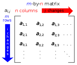
The horizontal and vertical lines in a matrix are called rows and columns, respectively. The numbers in the matrix are called its entries. To specify a matrix's size, a matrix with m rows and n columns is called an m-by-n matrix or m × n matrix. Such a matrix has order m × n. m and n are called its dimensions. The above is a 4-by-3 matrix.
A matrix where one of the dimensions equals one is also called a vector, and may be interpreted as an element of real coordinate space. An m × 1 matrix (one column and m rows) is called a column vector and a 1 × n matrix (one row and n columns) is called a row vector. For example, the second row vector of the above matrix is

Most of this article focusses on real and complex matrices, i.e., matrices whose entries are real or complex numbers. More general types of entries are discussed below.
[edit] Notation
The entry that lies in the i-th row and the j-th column of a matrix is typically referred to as the i,j, (i,j), or (i,j)th entry of the matrix. For example, (2,3) entry of the above matrix X is 7.
Matrices are usually denoted using upper-case letters, while the corresponding lower-case letters, with two subscript indices, represent the entries. For example, the (i, j)th entry of a matrix A is most commonly written as ai,j. Alternative notations for that entry are A[i,j] or Ai,j. In addition to using upper-case letters to symbolize matrices, many authors use a special typographical style, commonly boldface upright (non-italic), to further distinguish matrices from other variables. An alternate convention is to annotate matrices with their dimensions in small type underneath the symbol, for example,  for an m-by-n matrix.[citation needed] The set of all m-by-n matrices is denoted M(m, n).
A common shorthand is
- A = [ai,j]i=1,...,m; j=1,...,n or more briefly A = [ai,j]m×n
to define an m × n matrix A. In this case, the entries ai,j are defined separately for all integers 1 ≤ i ≤ m and 1 ≤ j ≤ n; for example the 2-by-2 matrix
is specified by A = [i − j]i=1,2; j=1,2
Some programming languages start the numbering of rows and columns at zero, in which case the entries of an m-by-n matrix are indexed by 0 ≤ i ≤ m − 1 and 0 ≤ j ≤ n − 1.[2] This article will follow the numerotation starting from 1.
[edit] History
Matrices have a long history of application in solving linear equations. The Chinese text from between 300 BC and AD 200, The Nine Chapters on the Mathematical Art (Jiu Zhang Suan Shu), is the first example of the use of matrix methods to solve simultaneous equations,[3] including the concept of determinants, almost 2000 years before its publication by the Japanese mathematician Seki Kowa in 1683 and the German mathematician Gottfried Leibniz in 1693.[citation needed]
Magic squares were known to Chinese mathematicians, as early as 650 BC[4] and Arab mathematicians, possibly as early as the 7th century, when the Arabs conquered northwestern parts of the Indian subcontinent and learned Indian mathematics and astronomy, including other aspects of combinatorial mathematics.[citation needed] It has also been suggested that the idea came via China. The first magic squares of order 5 and 6 appear in an encyclopedia from Baghdad circa 983 AD, the Encyclopedia of the Brethren of Purity (Rasa'il Ihkwan al-Safa); simpler magic squares were known to several earlier Arab mathematicians.[4]
The modern matrix concept started with linear algebra. Later, after the development of the theory of determinants by Seki Kowa and Leibniz in the late 17th century, Cramer developed the theory further in the 18th century, presenting Cramer's rule in 1750. Carl Friedrich Gauss and Wilhelm Jordan developed Gauss-Jordan elimination in the 1800s. The term "matrix" was coined in 1848 by J. J. Sylvester. Cayley, Hamilton, Grassmann, Frobenius and von Neumann are among the famous mathematicians who have worked on matrix theory.
[edit] Basic operations
There are a number of operations that can be applied to modify matrices called matrix addition, scalar multiplication and transposition.[5] These form the basic techniques to deal with matrices.
| Operation | Definition | Example |
|---|---|---|
| Addition | The sum A+B of two m-by-n matrices A and B is calculated entrywise:
|
|
| Scalar multiplication | The scalar multiplication cA of a matrix A and a number c (also called a scalar in the parlance of abstract algebra) is given by multiplying every entry of A by c:
|
 |
| Transpose | The transpose of an m-by-n matrix A is the n-by-m matrix AT (also denoted Atr or tA) formed by turning rows into columns and vice versa:
|
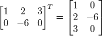 |

Familiar properties of numbers extend to these operations of matrices: for example, addition is commutative, i.e. the matrix sum does not depend on the order of the summands: A + B = B + A.[6] The transpose is compatible with addition and scalar multiplication, as expressed by (cA)T = c(AT) and (A + B)T = AT + BT. Finally, (AT)T = A.
[edit] Matrix multiplication, linear equations and linear transformations
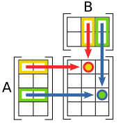
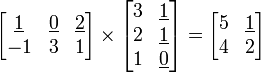
Multiplication of two matrices is defined only if the number of columns of the left matrix is the same as the number of rows of the right matrix. If A is an m-by-n matrix and B is an n-by-p matrix, then their matrix product AB is the m-by-p matrix whose entries are given by
![[\mathbf{AB}]_{i,j} = A_{i,1}B_{1,j} + A_{i,2}B_{2,j} + ... + A_{i,n}B_{n,j} = \sum_{r=1}^n A_{i,r}B_{r,j}](http://upload.wikimedia.org/math/4/2/0/42099b2d4839d839092d25d43a447c94.png)
where 1 ≤ i ≤ m and 1 ≤ j ≤ p.[7] For example (the highlighted entry 1 in the product is calculated as the product 1 · 1 + 0 · 1 + 2 · 0 = 1):
Matrix multiplication satisfies the rules (AB)C = A(BC) (associativity), and (A+B)C = AC+BC as well as C(A+B) = CA+CB (left and right distributivity), whenever the size of the matrices is such that the various products are defined.[8] The product AB may be defined without BA being defined, namely if A and B are m-by-n and n-by-k matrices, respectively, and m ≠ k. Even if both products are defined, they need not be equal, i.e. generally one has
- AB ≠ BA,
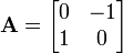
i.e. matrix multiplication is not commutative, in marked contrast to (rational, real, or complex) numbers whose product is independent of the order of the factors. An example for two matrices not commuting with each other is:  , whereas
The identity matrix In of size n is the n-by-n matrix in which all the elements on the main diagonal are equal to 1 and all other elements are equal to 0, e.g.
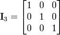
It is called identity matrix because multiplication with it leaves a matrix unchanged: MIn = ImM = M for any m-by-n matrix M.
Besides the ordinary matrix multiplication just described, there exist other less frequently used operations on matrices that can be considered forms of multiplication, such as the Hadamard product and the Kronecker product.[9] They arise in solving matrix equations such as the Sylvester equation.
[edit] Linear equations
A particular case of matrix multiplication is tightly linked to linear equations: if x designates a column vector (i.e. n×1-matrix) of n variables x1, x2, ..., xn, and A is an m-by-n matrix, then the matrix equation
- Ax = b, where b is some m×1-column vector
is equivalent to the system of linear equations
- A1,1x1 + A1,2x2 + ... + A1,nxn = b1
- ...
- Am,1x1 + Am,2x2 + ... + Am,nxn = bm[10]
This way, matrices can be used to compactly write and deal with multiple linear equations, i.e. systems of linear equations.
[edit] Linear transformations
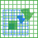
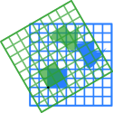
Matrices and matrix multiplication reveal their essential features when related to linear transformations (or linear maps). Any m-by-n matrix A gives rise to a linear transformation Rn → Rm, by assigning to any vector x in Rn the (matrix) product Ax, which is an element in Rm. Conversely, given any linear transformation, there exists a unique matrix A, such that the transformation is given by this formula: its (i, j)-entry ai,j is given by the i-th component of f(ej), where ej = (0, ..., 0, 1, 0, ..., 0) is the unit vector with 1 at the j-th spot and 0 elsewhere. The matrix A is said to represent the linear map f, and A is called the transformation matrix of f.
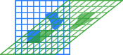
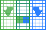
The following table shows a number of 2-by-2 matrices with the associated linear maps of R2. The blue original is mapped to the green grid and shapes, the origin (0, 0) is marked with a black point.
| Vertical shear with m=1.25. | Horizontal flip | Squeeze mapping with r=1.5 | Scaling by a factor of 1.5 | Rotation by π/6 = 30° |
 |
 |
 |
 |
 |
 |
 |
 |
 |
 |
Under the 1-to-1 correspondence of matrices and linear maps, matrix multiplication corresponds to composition of maps[11]: if a k-by-m matrix B represents another linear map g : Rm → Rk, then the composition g ∘ f is represented by BA since
- (g ∘ f)(x) = g(f(x)) = g(Ax) = B(Ax) = (BA)x.
The last equality follows from the above-mentioned associativity of matrix multiplication.
The nullity and rank of a matrix A are the dimension of the kernel and image of the linear map represented by A, respectively.[12] The rank is also characterized as the number of linear independent row vectors of the matrix, which is the same as the number of linear independent column vectors.[13] The sum of the nullity and rank equals the number of columns of the matrix, by the rank-nullity theorem.[14]
[edit] Square matrices
A square matrix is a matrix which has the same number of rows and columns. Due to this size restriction, all matrices can be multiplied (and added). A n-by-n matrix, also known as a square matrix of order n, A, is called invertible or non-singular if there exists a matrix B such that
- AB = In.[15]
This is equivalent to BA = In.[16] Moreover, if B exists, it is unique and is called the inverse matrix of A, denoted A−1.
The entries Ai,i form the main diagonal of a matrix. If all entries outside the main diagonal are zero, A is called diagonal matrix. If only all entries above (below) the main diagonal are zero, A is called a lower triangular matrix (upper triangular matrix, respectively). For example, if n = 3, they look like
 (diagonal),
  (lower) and
  (upper triangular matrix).
[edit] Determinant

The determinant det(A) or |A| of a square matrix A is a number encoding certain properties of the matrix. A matrix is invertible if and only if its determinant is nonzero. Its absolute value equals the area (in R2) or volume (in R3) of the image of the unit square (or cube), while its sign corresponds to the orientation of the corresponding linear map: the determinant is positive if and only if the orientation is preserved.
The determinant of 2-by-2 matrices is given by
 ,
,
the determinant of 3-by-3 matrices involves 6 terms (rule of Sarrus). The more lengthy Leibniz formula generalises these two formulae to all dimensions.[17]
The determinant of a product of matrices equals the product of the determinants: det(AB) = det(A) · det(B).[18] Adding multiples of rows or columns to other rows or columns does not change the determinant. Exchanging rows or columns alters the sign of the determinant.[19] Using these two operations, any matrix can be transformed to a lower (or upper) triangular matrix, whose determinant equals the product of the entries on the main diagonal; therefore the determinant of the original matrix can be calculated. Finally, the Laplace expansion expresses the determinant in terms of minors, i.e., determinants of smaller matrices.[20] Determinants can be used to solve linear systems using Cramer's rule, where the division of the determinants of two related square matrices equates to the value of each of the system's variables.[21]
[edit] Eigenvalues and eigenvectors
A number λ and a non-zero vector v satisfying
- Av = λv
are called eigenvalue and eigenvector of A, respectively.[nb 1][22] The number λ is an eigenvalue of A if and only if A−λIn is not invertible, which is equivalent to
- det(A−λI) = 0.[23]
The function pA(t) = det(A−tI) is called the characteristic polynomial of A, the degree of this polynomial is n. Therefore pA(t) has at most n (possibly complex) different roots, i.e. eigenvalues of the matrix.[24]
The trace of a square matrix is the sum of its diagonal entries. It equals the sum of its n eigenvalues.
[edit] Definiteness
| Matrix A; definiteness; associated bilinear form BA(v), v = (x, y); set of vectors v such that BA(v) |
|
 |
 |
| positive definite | indefinite |
| 1/4 x2 + y2 | 1/4 x2 − 1/4 y2 |
 Ellipse |
 Hyperbola |
A square matrix A that is equal to its transpose, i.e. A = AT, is a symmetric matrix; if it is equal to the negative of its transpose, i.e. A = −AT, then it is a skew-symmetric matrix. A symmetric n×n-matrix is called positive definite (negative definite, indefinite, resp.), if for all nonzero vectors x ∈ Rn the associated quadratic form given by
- Q(x) = xTAx
takes only positive values (negative, both negative and positive values, respectively).[25] Allowing as input two different vectors instead yields the bilinear form associated to A:
- BA (x, y) = xTAy.[26]
A matrix is positive definite if and only if all its eigenvalues are positive.[27] Definiteness can also be defined for complex Hermitian matrices, which satisfy A∗ = A, where the star denotes the conjugate transpose of the matrix, i.e. the transpose of the complex conjugate of A. The table at the right shows two possibilities for 2-by-2 matrices.
By the spectral theorem, positive definite matrices have an eigenbasis, i.e. every vector is expressible as a linear combination of eigenvectors. Also, all eigenvalues are real.[28]
[edit] Computational aspects
In addition to theoretical knowledge of properties of matrices and their relation to other fields, it is important for practical purposes to perform matrix calculations effectively and precisely. The domain studying these matters is called numerical linear algebra.[29] As with other numerical situations, two main aspects are the complexity of algorithms and their numerical stability. Many problems can be solved by both direct algorithms or iterative approaches. For example, finding eigenvectors can be done by finding a sequence of vectors xn converging to an eigenvector when n tends to infinity.[30]
Determining the complexity of an algorithm means finding upper bounds or estimates of how many elementary operations such as additions and multiplications of scalars are necessary to perform some algorithm, e.g. multiplication of matrices. For example, calculating the matrix product of two n-by-n matrix using the definition given above needs n3 multiplications, since for any of the n2 entries of the product, n multiplications are necessary. The Strassen algorithm outperforms this "naive" algorithm; it needs only n2.807 multiplications.[31] A refined approach also incorporates specific features of the computing devices.
In many practical situations additional information about the matrices involved is known. An important case are sparse matrices, i.e. matrices most of whose entries are zero. There are specifically adapted algorithms for, say, solving linear systems Ax = b for sparse matrices A, such as the conjugate gradient method.[32]
An algorithm is, roughly speaking, numerical stable, if little deviations (such as rounding errors) do not lead to big deviations in the result. For example, calculating the inverse of a matrix via Laplace's formula (Adj (A) denotes the adjugate matrix of A)
- A−1 = Adj(A) / det(A)
may lead to significant rounding errors if the determinant of the matrix is very small. The norm of a matrix can be used to capture the conditioning of linear algebraic problems, such as computing a matrix' inverse.[33]
Although most computer languages are not designed with commands or libraries for matrices, as early as the 1970s, some engineering desktop computers such as the HP 9830 had ROM cartridges to add BASIC commands for matrices. Some computer languages such as APL were designed to manipulate matrices, and various mathematical programs can be used to aid computing with matrices.[34]
[edit] Matrix decomposition methods
There are several methods to render matrices into a more easily accessible form. They are generally referred to as matrix transformation or matrix decomposition techniques. The interest of all these decomposition techniques is that they preserve certain properties of the matrices in question, such as determinant, rank or inverse, so that these quantities can be calculated after applying the transformation, or that certain matrix operations are algorithmically easier to carry out for some types of matrices.
The LU decomposition factors matrices as a product of lower (L) and an upper triangular matrices (U).[35] Once this decomposition is calculated, linear systems can be solved more efficiently, by a simple technique called forward and back substitution. Likewise, inverses of triangular matrices are algorithmically easier to calculate. The Gaussian elimination is a similar algorithm; it transforms any matrix to row echelon form.[36] Both methods proceed by multiplying the matrix by suitable elementary matrices, which correspond to permuting rows or columns and adding multiples of one row to another row.
The eigendecomposition expresses A as a product VDV−1, where D is a diagonal matrix and V is a suitable invertible matrix.[37] If A can be written in this form, it is called diagonalizable. More generally, and applicable to all matrices, the Jordan decomposition transforms a matrix into Jordan normal form.[38] Given the eigendecomposition, the nth power of A (i.e. n-fold iterated matrix multiplication) can be calculated via
- An = (VDV−1)n = VDV−1VDV−1...VDV−1 = VDnV−1
and the power of a diagonal matrix can be calculated by taking the corresponding powers of the diagonal entries, which is much easier than doing the exponentiation for A instead. This can be used to compute the matrix exponential eA, a need frequently arising in solving linear differential equations, matrix logarithms and square roots of matrices.[39] To avoid numerically ill-conditioned situations, further algorithms such as the Schur decomposition can be employed.[40]
The QR decomposition expresses a matrix as the product of an orthogonal matrix and a upper triangular matrix. It can be used for the QR algorithm, one of several algorithms computing the eigenvalues of a matrix.[41]
[edit] Abstract algebraic aspects and generalizations
[edit] Matrices with more general entries
This article focuses on matrices whose entries are real or complex numbers. However, matrices can be considered with much more general types of entries than real or complex numbers. As a first step of generalization, any field, i.e. a set where addition, subtraction, multiplication and division operations are defined and well-behaved, may be used instead of R or C, for example rational numbers or finite fields. Wherever eigenvalues are considered, the choice of the field usually matters insofar as a the characteristic polynomial, despite having real coefficients may have complex solutions. Therefore, the field is often required to be C or any algebraically closed field when such issues arise.
More generally, abstract algebra makes great use of matrices with entries in a ring R.[42] Rings are a more general notion than fields in that no division operation exists. The very same addition and multiplication operations of matrices extend to this setting, too. The set M(n, R) of all square n-by-n matrices over R is a ring in its own right, isomorphic to the endomorphism ring of the left R-module Rn.[43] If the ring R is commutative, i.e., its multiplication is commutative, then M(n, R) is a unitary noncommutative (unless n = 1) associative algebra over R. The determinant of square matrices can still be defined using the Leibniz formula; a matrix is invertible if and only if its determinant is invertible in R, generalising the situation over a field F, where every nonzero element is invertible.[44] Matrices over superrings are called supermatrices.[45]
[edit] Relationship to linear maps
Linear maps Rn → Rm are equivalent to n-by-m matrices, as described above. More generally, any linear map f: V → W between finite-dimensional vector spaces can be described by a matrix A = (aij), by choosing bases v1, ..., vm, and w1, ..., wn, where m and n are the dimensions of V and W, respectively, and requiring
 .
.
This uniquely determines the entries of the matrix A, but the matrix depends on the choice of the bases: different choices of bases give rise to different, but similar matrices.[46] Many of the above concrete notions can be reinterpreted in this light, for example, the transpose matrix AT describes the transpose of the linear map given by A, with respect to the dual bases.[47]
[edit] Infinite matrices
It is also possible to consider matrices with infinitely many rows and/or columns.[48] The basic operations introduced above are defined the same way in this case. Matrix multiplication, however, and all operations stemming therefrom are only meaningful when restricted to certain matrices, since the sum featuring in the above definition of the matrix product will contain an infinity of summands. An easy way to circumvent this issue is to restrict to matrices all of whose rows (or columns) contain only finitely many nonzero terms. As in the finite case (see above), where matrices describe linear maps, infinite matrices can be used to describe operators on Hilbert spaces, where convergence and continuity questions arise. However, the explicit point of view of matrices tends to obfuscate the matter,[nb 2] and the abstract and more powerful tools of functional analysis are used instead, by relating matrices to linear maps (as in the finite case above), but imposing additional convergence and continuity constraints.
[edit] Tensors
A vector can be seen as a sequence of numbers, a matrix is a rectangular or two-dimensional array of numbers. Extending this leads to tensors which can be seen as higher-dimensional arrays of numbers.[49]
[edit] Matrix groups
A group is a mathematical structure consisting of a set of objects together with a binary operation, i.e. an operation combining any two objects to a third, subject to certain requirements.[50] A group in which the objects are matrices and the group operation is matrix multiplication is called a matrix group.[nb 3][51] Since in a group every element has to be invertible, the most general matrix groups are the groups of all invertible matrices of a given size, called the general linear groups.
Any property of matrices that is preserved under matrix products and inverses can be used to define further matrix groups. For example, matrices with a given size and with a determinant of 1 form a subgroup of (i.e. a smaller group contained in) their general linear group, called a special linear group.[52] Orthogonal matrices, determined by the condition
- MTM = I
form the orthogonal group.[53] They are called orthogonal since the associated linear transformations of Rn preserve angles in the sense that the scalar product of two vectors is unchanged after applying M to them:
- (Mv) · (Mw) = v · w.[54]
Every finite group is isomorphic to a matrix group.[citation needed] General groups can be studied using matrix groups, which are comparatively well-understood, by means of representation theory.[55]
[edit] Applications
There are numerous applications of matrices, both in mathematics and other sciences. Some of them merely take advantage of the compact representation of a set of numbers in a matrix. For example, in game theory, the payoff matrix encodes the payoff for two players, depending on which out of a given (finite) set of alternatives the players choose.[56] Text mining and automatated thesaurus compilation makes use of document-term matrices such as tf-idf in order to keep track of frequencies of certain words in several documents.[57]
Complex numbers can be represented by particular real 2-by-2 matrices via
 ,
,
under which addition and multiplication of complex numbers and matrices correspond to each other. For example, 2-by-2 rotation matrices represent the multiplication with some complex number of absolute value 1, as above. A similar interpretation is possible for quaternions.[58]
Matrices over a polynomial ring are important in the study of control theory.
Early encryption techniques such as the Hill cipher also used matrices. However, due to the linear nature of matrices, these codes are comparatively easy to break.[59] Computer graphics uses matrices both to respresent objects and to calculate transformations of objects using affine rotation matrices to accomplish tasks such as projecting a three-dimensional object onto a two-dimensional screen, corresponding to a theoretical camera observation.[60]
[edit] Graph theory

 .
.The adjacency matrix of a finite graph is a basic notion of graph theory.[61] It saves which vertices of the graph are connected by an edge. Matrices containing just two different values (0 and 1 meaning for example "yes" and "no") are called logical matrices. The distance (or cost) matrix contains information about distances of the edges.[62] These concepts can be applied to websites connected hyperlinks or cities connected by roads etc., in which case (unless the road network is extremely dense) the matrices tend to be sparse, i.e. contain few nonzero entries. Therefore, specifically taylored matrix algorithms can be used in network theory.
[edit] Analysis and geometry
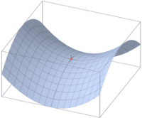
 is indefinite.
The Hessian matrix of a differentiable function f: Rn → R consists of the second derivatives of f with respect to the several coordinate directions, i.e.
![H(f) = \left [\frac {\partial^2f}{\partial x_i \partial x_j} \right ]](http://upload.wikimedia.org/math/1/9/0/1902b3309ca28eb311bf12bbf2a0a366.png) .[63]
.[63]
It encodes information about the local growth behaviour of the function: given a critical point x = (x1, ..., xn), i.e., a point where the first partial derivatives  of f vanish, the function has a local minimum if the Hessian matrix is positive definite. Quadratic programming can be used to find global minima or maxima of quadratic functions closely related to the ones attached to matrices (see above).[citation needed]
Another matrix frequently used in geometrical situations is the Jacobi matrix of a differentiable map f: Rn → Rm. If f1, ..., fm denote the components of f, then the Jacobi matrix is defined as
![J(f) = \left [\frac {\partial f_i}{\partial x_j} \right ]_{1 \leq i \leq m, 1 \leq j \leq n}](http://upload.wikimedia.org/math/d/8/f/d8f569179d6057a7897dd493aee858c6.png) .[64]
.[64]
If n > m, and if the rank of the Jacobi matrix attains its maximal value m, f is locally invertible at that point, by the implicit function theorem.[65]
Partial differential equations can be classified by considering the matrix of coefficients of the highest-order differential operators of the equation. For elliptic partial differential equations this matrix is positive definite, which has decisive influence on the set of possible solutions of the equation in question.[66]
The finite element method is an important numerical method to solve partial differential equations, widely applied in simulating complex physical systems. It attempts to approximate the solution to some equation by piecewise linear functions, where the pieces are chosen with respect to a sufficiently fine grid, which in turn can be recast as a matrix equation.[67]
[edit] Probability theory and statistics

 (red) and
  (black).
Stochastic matrices are square matrices whose rows are probability vectors, i.e., whose entries sum up to one. Stochastic matrices are used to define Markov chains with finitely many states.[68] A row of the stochastic matrix gives the probability distribution for the next position of some particle which is currently in the state corresponding to the row. Properties of the Markov chain like absorbing states, i.e. states that any particle attains eventually, can be read off the eigenvectors of the transition matrices.[69]
Statistics also makes use of matrices in many different forms. Descriptive statistics is concerned with describing data sets, which can often be represented in matrix form, by reducing the amount of data. The covariance matrix encodes the mutual variance of several random variables.[70] Another technique using matrices are linear least squares, a method that approximates a finite set of pairs (x1, y1), (x2, y2), ..., (xN, yN), by a linear function
- yi ≈ axi + b, i = 1, ..., N
which can be formulated in terms of matrices, related to the singular value decomposition of matrices.[71]
Random matrices are matrices whose entries are random numbers, subject to suitable probability distributions, such as matrix normal distribution. Beyond probability theory, they are applied in domains ranging from number theory to physics.[72][73]
[edit] Symmetries and transformations in physics
Linear transformations and the associated symmetries play a key role in modern physics. For example, elementary particles in quantum field theory are classified as representations of the Lorentz group of special relativity and, more specifically, by their behavior under the spin group. Concrete representations involving the Pauli matrices and more general gamma matrices are an integral part of the physical description of fermions, which behave as spinors.[74] For the three lightest quarks, there is a group-theoretical representation involving the special unitary group SU(3); for their calculations, physicists use a convenient matrix representation known as the Gell-Mann matrices, which are also used for the SU(3) gauge group that forms the basis of the mordern description of strong nuclear interactions, quantum chromodynamics. The Cabibbo-Kobayashi-Maskawa matrix, in turn, expresses the fact that the basic quark states that are important for weak interactions are not the same as, but linearly related to the basic quark states that define particles with specific and distinct masses.[75]
[edit] Linear combinations of quantum states
The first model of quantum mechanics (Heisenberg, 1925) represented the theory's operators by infinite-dimensional matrices acting on quantum states.[76] This is also referred to as matrix mechanics. One particular example is the density matrix that characterizes the "mixed" state of a quantum system as a linear combination of elementary, "pure" eigenstates.[77]
Another matrix serves as a key tool for describing the scattering experiments which form the cornerstone of experimental particle physics: Collision reactions such as occur in particle accelerators, where non-interacting particles head towards each other and collide in a small interaction zone, with a new set of non-interacting particles as the result, can be described as the scalar product of outgoing particle states and a linear combination of ingoing particle states. The linear combination is given by a matrix known as the S-matrix, which encodes all information about the possible interactions between particles.[78]
[edit] Normal Modes
A general application of matrices in physics is to the description of linearly coupled harmonic systems. The equations of motion of such systems can be described in matrix form, with a mass matrix multiplying a generalized velocity to give the kinetic term, and a force matrix multiplying a displacement vector to characterize the interactions. The best way to obtain solutions is to determine the system's eigenvectors, its normal modes, by diagonalizing the matrix equation. Techniques like this are crucial when it comes to describing the internal dynamics of molecules: the internal vibrations of systems consisting of mutually bound component atoms.[79] They are also needed for describing mechanical vibrations, and oscillations in electrical circuits.[80]
[edit] Geometrical optics
Geometrical optics provides further matrix applications. In this approximative theory, the wave nature of light is neglected. The result is a model in which light rays are indeed geometrical rays. If the deflection of light rays by optical elements is small, the action of a lens or reflective element on a given light ray can be expressed as multiplication of a two-component vector with a two-by-two matrix called ray transfer matrix: the vector's components are the light ray's slope and its distance from the optical axis, while the matrix encodes the properties of the optical element. The matrix characterizing an optical system consisting of a combination of lenses and/or reflective elements is simply the product of the components' matrices.[81]
[edit] Computational neuroscience
Some computational models of how the brain could store information (and to which some liken certain hippocampal circuits) are based on correlation matrices. For an example, see McNaughton 1989.
[edit] See also
| The Wikibook Linear Algebra has a page on the topic of |
| Wikiversity has learning materials about Matrices at: |
[edit] Footnotes
- ^ Brown 1991, Chapter I.1. Alternative references for this book include Lang 1987b and Greub 1975.
- ^ Oualline 2003, Ch. 5.
- ^ Shen Kangshen et al. (ed.) (1999). Nine Chapters of the Mathematical Art, Companion and Commentary. Oxford University Press. cited by Otto Bretscher (2005). Linear Algebra with Applications (3rd ed. ed.). Prentice-Hall. pp. p. 1.
- ^ a b Swaney, Mark. History of Magic Squares.
- ^ Brown 1991, Definition I.2.1 (addition), Definition I.2.4 (scalar multiplication), and Definition I.2.33 (transpose)
- ^ Brown 1991, Theorem I.2.6.
- ^ Brown 1991, Definition I.2.20.
- ^ Brown 1991, Theorem I.2.24.
- ^ Horn & Johnson 1985, Ch. 4 and 5.
- ^ Brown 1991, I.2.21 and 22.
- ^ Greub 1975, Section III.2.
- ^ Greub 1975, Section III.1.
- ^ Brown 1991, Definition II.3.3.
- ^ Brown 1991, Theorem II.3.22.
- ^ Brown 1991, Definition I.2.28.
- ^ Brown 1991, Definition I.5.13.
- ^ Brown 1991, Definition III.2.1.
- ^ Brown 1991, Theorem III.2.12.
- ^ Brown 1991, Corollary III.2.16.
- ^ Mirsky 1990, Theorem 1.4.1.
- ^ Brown 1991, Theorem III.3.18.
- ^ Brown 1991, Definition III.4.1.
- ^ Brown 1991, Definition III.4.9.
- ^ Brown 1991, Corollary III.4.10.
- ^ Horn & Johnson 1985, Chapter 7.
- ^ Horn & Johnson 1985, Example 4.0.6, p. 169.
- ^ Horn & Johnson 1985, Theorem 7.2.1.
- ^ Horn & Johnson 1985, Theorem 2.5.6.
- ^ Bau III & Trefethen 1997.
- ^ Householder 1975, Ch. 7.
- ^ Golub & Van Loan 1996, Algorithm 1.3.1.
- ^ Golub & Van Loan 1996, Chapters 9 and 10, esp. section 10.2.
- ^ Golub & Van Loan 1996, Chapter 2.3.
- ^ For example, Mathematica, see Wolfram (2003).
- ^ Press, Flannery & Teukolsky 1992.
- ^ Stoer & Bulirsch 2002, Section 4.1.
- ^ Horn & Johnson 1985, Theorem 2.5.4.
- ^ Horn & Johnson 1985, Ch. 3.1, 3.2.
- ^ Arnold & Cooke 1992, Sections 14.5, 7, 8.
- ^ Bronson 1989, Ch. 15.
- ^ Stoer & Bulirsch 2002, Section 4.7.
- ^ Lang 2002, Chapter XIII.
- ^ Lang 2002, XVII.1, p. 643.
- ^ Lang 2002, Proposition XIII.4.16.
- ^ Reichl 2004, Section L.2.
- ^ Greub 1975, Section III.3.
- ^ Greub 1975, Section III.3.13.
- ^ See the item "Matrix" in Itõ, ed. 1987.
- ^ Coburn 1955, Ch. V.
- ^ See any standard reference in group.
- ^ Baker 2003, Def. 1.30.
- ^ Baker 2003, Theorem 1.2.
- ^ Artin 1991, Chapter 4.5.
- ^ Artin 1991, Theorem 4.5.13.
- ^ See any reference in representation theory or group representation.
- ^ Fudenberg & Tirole 1983, Section 1.1.1.
- ^ Manning 1999, Section 15.3.4.
- ^ Ward 1997, Ch. 2.8.
- ^ Stinson 2005, Ch. 1.1.5 and 1.2.4.
- ^ Association for Computing Machinery 1979, Ch. 7.
- ^ Godsil & Royle 2004, Ch. 8.1.
- ^ Punnen 2002.
- ^ Lang 1987a, Ch. XVI.6.
- ^ Lang 1987a, Ch. XVI.1.
- ^ Lang 1987a, Ch. XVI.5. For a more advanced, and more general statement see Lang 1969, Ch. VI.2.
- ^ Gilbarg & Trudinger 2001.
- ^ Šolin 2005, Ch. 2.5. See also stiffness method.
- ^ Latouche & Ramaswami 1999.
- ^ Mehata & Srinivasan 1978, Ch. 2.8.
- ^ Krzanowski 1988, Ch. 2.2., p. 60.
- ^ Krzanowski 1988, Ch. 4.1.
- ^ Conrey 2007.
- ^ Zabrodin, Brezin & Kazakov et al. 2006.
- ^ Itzykson & Zuber 1980, Ch. 2.
- ^ see Burgess & Moore 2007, section 1.6.3. (SU(3)), section 2.4.3.2. (Kobayashi-Maskawa matrix).
- ^ Schiff 1968, Ch. 6.
- ^ Bohm 2001, sections II.4 and II.8.
- ^ Weinberg 1995, Ch. 3.
- ^ Wherrett 1987, part II.
- ^ Riley, Hobson & Bence 1997, 7.17.
- ^ Guenther 1990, Ch. 5.
[edit] References
- Arnold, V. I.; Cooke, Roger (1992), Ordinary differential equations, Berlin, New York: Springer-Verlag, ISBN 978-3-540-54813-3
- Artin, Michael (1991), Algebra, Prentice Hall, ISBN 978-0-89871-510-1
- Association for Computing Machinery (1979), Computer Graphics, Tata McGraw-Hill, ISBN 978-0-07-059376-3
- Baker, Andrew J. (2003), Matrix Groups: An Introduction to Lie Group Theory, Berlin, New York: Springer-Verlag, ISBN 978-1-85233-470-3
- Bau III, David; Trefethen, Lloyd N. (1997), Numerical linear algebra, Philadelphia: Society for Industrial and Applied Mathematics, ISBN 978-0-89871-361-9
- Bronson, Richard (1989), Schaum's outline of theory and problems of matrix operations, New York: McGraw-Hill, ISBN 978-0-07-007978-6
- Brown, William A. (1991), Matrices and vector spaces, New York: M. Dekker, ISBN 978-0-8247-8419-5
- Coburn, Nathaniel (1955), Vector and tensor analysis, New York: Macmillan, OCLC 1029828
- Conrey, J. B. (2007), Ranks of elliptic curves and random matrix theory, Cambridge University Press, ISBN 978-0-521-69964-8
- Fudenberg, D.; Tirole, Jean (1983), Game Theory, MIT Press
- Gilbarg, David; Trudinger, Neil S. (2001), Elliptic partial differential equations of second order (2nd ed.), Berlin, New York: Springer-Verlag, ISBN 978-3-540-41160-4
- Godsil, Chris; Royle, Gordon (2004), Algebraic Graph Theory, Graduate Texts in Mathematics, 207, Berlin, New York: Springer-Verlag, ISBN 978-0-387-95220-8
- Golub, Gene H.; Van Loan, Charles F. (1996), Matrix Computations (3rd ed.), Johns Hopkins, ISBN 978-0-8018-5414-9
- Greub, Werner Hildbert (1975), Linear algebra, Graduate Texts in Mathematics, Berlin, New York: Springer-Verlag, ISBN 978-0-387-90110-7
- Halmos, Paul Richard (1982), A Hilbert space problem book, Graduate Texts in Mathematics, 19 (2nd ed.), Berlin, New York: Springer-Verlag, MR675952, ISBN 978-0-387-90685-0
- Horn, Roger A.; Johnson, Charles R. (1985), Matrix Analysis, Cambridge University Press, ISBN 978-0-521-38632-6
- Householder, Alston S. (1975), The theory of matrices in numerical analysis, New York: Dover Publications, MR0378371
- Krzanowski, W. J. (1988), Principles of multivariate analysis, Oxford Statistical Science Series, 3, The Clarendon Press Oxford University Press, MR969370, ISBN 978-0-19-852211-9
- Itõ, Kiyosi, ed. (1987), Encyclopedic dictionary of mathematics. Vol. I--IV (2nd ed.), MIT Press, MR901762, ISBN 978-0-262-09026-1
- Lang, Serge (1969), Analysis II, Addison-Wesley
- Lang, Serge (1987a), Calculus of several variables (3rd ed.), Berlin, New York: Springer-Verlag, ISBN 978-0-387-96405-8
- Lang, Serge (1987b), Linear algebra, Berlin, New York: Springer-Verlag, ISBN 978-0-387-96412-6
- Lang, Serge (2002), Algebra, Graduate Texts in Mathematics, 211 (Revised third ed.), New York: Springer-Verlag, MR1878556, ISBN 978-0-387-95385-4
- Latouche, G.; Ramaswami, V. (1999), Introduction to matrix analytic methods in stochastic modeling (1st ed.), Philadelphia: Society for Industrial and Applied Mathematics, ISBN 978-0-89871-425-8
- Manning, Christopher D.; Schütze, Hinrich (1999), Foundations of statistical natural language processing, MIT Press, ISBN 978-0-262-13360-9
- Mehata, K. M.; Srinivasan, S. K. (1978), Stochastic processes, New York: McGraw-Hill, ISBN 978-0-07-096612-3
- Mirsky, Leonid (1990), An Introduction to Linear Algebra, Courier Dover Publications, ISBN 978-0-486-66434-7, http://books.google.de/books?id=ULMmheb26ZcC&pg=PA1&dq=linear+algebra+determinant&lr=lang_en&as_brr=3&as_pt=ALLTYPES#PPA16,M1
- Oualline, Steve (2003), Practical C++ programming, O'Reilly, ISBN 978-0-596-00419-4
- Press, William H.; Flannery, Brian P.; Teukolsky, Saul A.; Vetterling, William T. (1992), "LU Decomposition and Its Applications", Numerical Recipes in FORTRAN: The Art of Scientific Computing (2nd ed.), Cambridge University Press, pp. 34–42, http://www.mpi-hd.mpg.de/astrophysik/HEA/internal/Numerical_Recipes/f2-3.pdf
- Punnen, Abraham P.; Gutin, Gregory (2002), The traveling salesman problem and its variations, Boston: Kluwer Academic Publishers, ISBN 978-1-4020-0664-7
- Reichl, Linda E. (2004), The transition to chaos: conservative classical systems and quantum manifestations, Berlin, New York: Springer-Verlag, ISBN 978-0-387-98788-0
- Šolin, Pavel (2005), Partial Differential Equations and the Finite Element Method, Wiley-Interscience, ISBN 978-0-471-76409-0
- Stinson, Douglas R. (2005), Cryptography, Discrete Mathematics and Its Applications, Chapman & Hall/CRC, ISBN 978-1-58488-508-5
- Stoer, Josef; Bulirsch, Roland (2002), Introduction to Numerical Analysis (3rd ed.), Berlin, New York: Springer-Verlag, ISBN 978-0-387-95452-3
- Ward, J. P. (1997), Quaternions and Cayley numbers, Mathematics and its Applications, 403, Dordrecht: Kluwer Academic Publishers Group, MR1458894, ISBN 978-0-7923-4513-8
- Wolfram, Stephen (2003), The Mathematica Book (5th ed.), Champaign, Ill: Wolfram Media, ISBN 978-1-57955-022-6
[edit] Physics references
- Bohm, Arno (2001), Quantum Mechanics: Foundations and Applications, Springer, ISBN 0-387-95330-2
- Burgess, Cliff; Moore, Guy (2007), The Standard Model. A Primer, Cambridge University Press, ISBN 0-521-86036-9
- Guenther, Robert D. (1990), Modern Optics, John Wiley, ISBN 0-471-60538-7
- Itzykson, Claude; Zuber, Jean-Bernard (1980), Quantum Field Theory, McGraw-Hill, ISBN 0-07-032071-3
- Riley, K. F.; Hobson, M. P.; Bence, S. J. (1997), Mathematical methods for physics and engineering, Cambridge University Press, ISBN 0-521-55506-X
- Schiff, Leonard I. (1968), Quantum Mechanics (3rd ed.), McGraw-Hill
- Weinberg, Steven (1995), The Quantum Theory of Fields. Volume I: Foundations, Cambridge University Press, ISBN 0-521-55001-7
- Wherrett, Brian S. (1987), Group Theory for Atoms, Molecules and Solids, Prentice-Hall International, ISBN 0-13-365461-3
- Zabrodin, Anton; Brezin, Édouard; Kazakov, Vladimir; Serban, Didina; Wiegmann, Paul (2006), Applications of Random Matrices in Physics (NATO Science Series II: Mathematics, Physics and Chemistry), Berlin, New York: Springer-Verlag, ISBN 978-1-4020-4530-1
[edit] External links
- History
- MacTutor: Matrices and determinants
- Matrices and Linear Algebra on the Earliest Uses Pages
- Earliest Uses of Symbols for Matrices and Vectors
- Online books
- Kaw, Autar K., Introduction to Matrix Algebra, ISBN 978-0-615-25126-4, http://autarkaw.com/books/matrixalgebra/index.html
- The Matrix Cookbook, http://matrixcookbook.com, retrieved on 12/10/2008
- Brookes, M. (2005), The Matrix Reference Manual, London: Imperial College, http://www.ee.ic.ac.uk/hp/staff/dmb/matrix/intro.html, retrieved on 12/10/2008
- Online Matrix Calculators
- Xiao, Gang, Matrix calculator, http://wims.unice.fr/wims/wims.cgi?module=tool/linear/matrix.en, retrieved on 12/10/2008
- Online matrix calculator, http://www.bluebit.gr/matrix-calculator/, retrieved on 12/10/2008
- Oehlert, Gary W.; Bingham, Christopher, MacAnova, University of Minnesota, School of Statistics, http://www.stat.umn.edu/macanova/macanova.home.html, retrieved on 12/10/2008, a freeware package for matrix algebra and statistics

