Weighted mean

From Wikipedia, the free encyclopedia

The weighted mean is similar to an arithmetic mean (the most common type of average), where instead of each of the data points contributing equally to the final average, some data points contribute more than others. The notion of weighted mean plays a role in descriptive statistics and also occurs in a more general form in several other areas of mathematics.

If all the weights are equal, then the weighted mean is the same as the arithmetic mean. While weighted means generally behave in a similar fashion to arithmetic means, they do have a few counter-intuitive properties, as captured for instance in Simpson's paradox.

The term weighted average usually refers to a weighted arithmetic mean, but weighted versions of other means can also be calculated, such as the weighted geometric mean and the weighted harmonic mean.

1 Example
2 Mathematical definition
3 Length-weighted mean
4 Convex combination
5 Statistical properties
6 Dealing with variance
- 6.1 Correcting for over/under dispersion
7 Weighted sample variance
8 Accounting for correlations
9 Decreasing strength of interactions
10 Exponentially decreasing weights
11 See also
12 References
13 External links

[edit] Example

Given two school classes, one with 20 students, and one with 30 students, the grades in each class on a test were:

Morning class = 62, 67, 71, 74, 76, 77, 78, 79, 79, 80, 80, 81, 81, 82, 83, 84, 86, 89, 93, 98

Afternoon class = 81, 82, 83, 84, 85, 86, 87, 87, 88, 88, 89, 89, 89, 90, 90, 90, 90, 91, 91, 91, 92, 92, 93, 93, 94, 95, 96, 97, 98, 99

The straight average for the morning class is 80 and the straight average of the afternoon class is 90. The straight average of 80 and 90 is 85, the mean of the two class means. However, this does not account for the difference in number of students in each class, and the value of 85 does not reflect the average student grade (independent of class). The average student grade can be obtained by either averaging all the numbers without regard to classes, or weighting the class means by the number of students in each class:

$\bar{x} = \frac{4300}{50} = 86.$

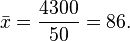
Or, using a weighted mean of the class means:

$\bar{x} = \frac{(20)80 + (30)90}{20 + 30} = 86.$

The weighted mean makes it possible to find the average student grade also in the case where only the class means and the number of students in each class are available.

[edit] Mathematical definition

Formally, the weighted mean of a non-empty set of data

$[x_1, x_2, \dots , x_n]\,,$

with non-negative weights

$[w_1, w_2, \dots, w_n]\,,$

is the quantity calculated by

$\bar{x} = \frac{ \sum_{i=1}^n w_i x_i}{\sum_{i=1}^n w_i},$

which means:

$\bar{x} = \frac{w_1 x_1 + w_2 x_2 + \cdots + w_n x_n}{w_1 + w_2 + \cdots + w_n}.$

So data elements with a high weight contribute more to the weighted mean than do elements with a low weight. The weights must not be negative. They may be zero, but not all of them (because division by zero is not allowed).

Formulae and calculations become much simpler when normalizing the weights, such that they sum up to $1$ , i.e. $\sum_{i=1}^n {w_i} = 1$ . Normalized weights are easily obtained by dividing each weight by the sum of all weights, $V_1=\sum_{i=1}^n {w_i}$ , i.e. by the re-definition $w_i = \frac {w_i}{V_1}$ . For normalized weights the weighted mean is simply $\bar {x} = \sum_{i=1}^n {w_i x_i}$ .

The common mean $\frac {\sum_{i=1}^n {x_i}} {n}$ results as a special case of the weighted mean when all data have equal weights, that is when $w i = w$ .

[edit] Length-weighted mean

For weighting a response variable based upon its dependency on x, a distance variable.

$\bar{y} = \frac{y_2 x_2 - y_1 x_1}{x_2 - x_1}$

[edit] Convex combination

Since only the relative weights are relevant, any weighted mean can be expressed using coefficients that sum to one. Such a linear combination is called a convex combination.

Using the previous example, we would get the following:

$\frac{20}{20 + 30} = 0.4\,$

$\frac{30}{20 + 30} = 0.6\,$

$\bar{x} = \frac{(0.4)80\% + (0.6)90\%}{0.4 + 0.6} = 86\%.$

This simplifies to:

$\bar{x} = (0.4)80\% + (0.6)90\% = 86\%.$

[edit] Statistical properties

The weighted sample mean $\bar{x}$ with normalized weights is itself a random variable. How are its expected value and standard deviation related to the expected values and standard deviations of the observations?

If the observations have expected values $E(x_i )=\bar {x_i}$ , then the weighted sample mean has expectation $E(\bar{x}) = \sum_{i=1}^n {w_i \bar{x_i}}$ . Particularly, if the expectations of all observations are equal, $\bar {x_i}=c$ , then the expectation of the weighted sample mean is the same, $E(\bar{x})= c$ .

If the observations have standard deviations $σ i$ and are uncorrelated from each other, then the weighted sample mean has standard deviation 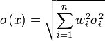$\sigma(\bar x)= \sqrt {\sum_{i=1}^n {w_i^2 \sigma^2_i}}$ . If moreover the standard deviations of all observations are equal, $σ i = d$ , then the weighted sample mean has standard deviation $\sigma(\bar x)= d \sqrt {V_2}$ , where $V 2$ is the interesting quantity $V_2=\sum_{i=1}^n {w_i^2}$ , which is lying in the range $1/n \le V_2\le 1$ . It attains the minimum for equal weights, and the maximum when all weights except one are zero. In the former case we have 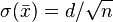$\sigma(\bar x)=d/ \sqrt {n}$ , which textbooks display in the chapter about the central limit theorem.

[edit] Dealing with variance

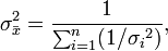
For the weighted mean of a list of data for which each element $x_i\,\!$ comes from a different probability distribution with known variance ${\sigma_i}^2\,$ , one possible choice for the weights is given by:

$w_i = \frac{1}{\sigma_i^2}.$

The weighted mean in this case is:

$\bar{x} = \frac{ \sum_{i=1}^n (x_i/{\sigma_i}^2)}{\sum_{i=1}^n (1/{\sigma_i}^2)},$

and the variance of the weighted mean is:

$\sigma_{\bar{x}}^2 = \frac{ 1 }{\sum_{i=1}^n (1/{\sigma_i}^2)},$

which reduces to $\sigma_{\bar{x}}^2 = \frac{ {\sigma_0}^2 }{n}$ , when all $\sigma_i = \sigma_0.\,$

The significance of this choice is that this weighted mean is the maximum likelihood estimator of the mean of the probability distributions under the assumption that they are independent and normally distributed with the same mean.

[edit] Correcting for over/under dispersion

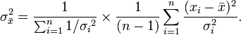
Weighted means are typically used to find the weighted mean of experimental data, rather than theoretically generated data. In this case, there will be some error in the variance of each data point. Typically experimental errors are underestimated because the experimenter does not know all sources of error in calculating the variance of each data point. In this event, the variance in the weighted mean must be corrected to account for the fact that $χ 2$ is too large. The correction that must be made is

$\sigma_{\bar{x}}^2 \rightarrow \sigma_{\bar{x}}^2 \chi^2_\nu$

where $\chi^2_\nu,$ is $χ 2,$ divided by the number of degrees of freedom, in this case $n - 1,$ . This gives the variance in the weighted mean as:

$\sigma_{\bar{x}}^2 = \frac{ 1 }{\sum_{i=1}^n 1/{\sigma_i}^2} \times \frac{1}{(n-1)} \sum_{i=1}^n \frac{ (x_i - \bar{x} )^2}{ \sigma_i^2 }.$

[edit] Weighted sample variance

Typically when you calculate a mean it is important to know the variance and standard deviation of that mean. When a weighted mean $μ *$ with normalized weights is used, the variance of the weighted sample is different from the variance of the unweighted sample. The biased weighted sample variance is defined similarly to the normal biased sample variance:

$\sigma^2\ = \frac{ \sum_{i=1}^N{\left(x_i - \mu\right)^2} }{ N }$

$\sigma^2_{weighted} \ = \sum_{i=1}^N{{w_i}\left(x_i - \mu^*\right)^2}$

For small sample of populations, it is customary to use an unbiased estimator for the population variance. In normal unweighted samples, the N in the denominator (corresponding to the sample size) is changed to N − 1. While this is simple in unweighted samples, it becomes tedious for weighted samples. Thus, the unbiased estimator of weighted population variance is given by [1]:

$s^2\ = \frac {1} {1-V_2} \sum_{i=1}^N{{w_i}\left(x_i - \mu^*\right)^2}$ ,

where $V 2$ was introduced in a previous section. The degrees of freedom of the weighted, unbiased sample variance vary accordingly from $N - 1$ down to $0$ .

The standard deviation is simply the square root of the variance above.

[edit] Accounting for correlations

In the general case, suppose that $\mathbf{X}=[x_1,\dots,x_n]$ , $\mathbf{C}$ is the covariance matrix relating the quantities $x i$ , $\bar{x}$ is the common mean to be estimated, and $\mathbf{W}$ is the design matrix [1, ..., 1] (of length n). The Gauss–Markov theorem says that the estimate of the mean having minimum variance is given by:

$\sigma^2_\bar{x}=(\mathbf{W}^T \mathbf{C}^{-1} \mathbf{W})^{-1},$

and

$\bar{x} = \sigma^2_\bar{x} (\mathbf{W}^T \mathbf{C}^{-1} \mathbf{X}).$

[edit] Decreasing strength of interactions

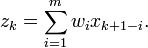
Consider the time series of an independent variable $x$ and a dependent variable $y$ , with $n$ observations sampled at discrete times $t i$ . In many common situations, the value of $y$ at time $t i$ depends not only from $x i$ but also from its past values. It is again most common, that the strength of this dependence decreases as the distance in time increases. To model this situation, one may replace the independent variable by its sliding mean $z$ with window size $m$ .

$z_k=\sum_{i=1}^m{{w_i}x_{k+1-i}}.$

Range Weighted Mean Interpretation
Weighted Mean Equivalence	Range (1-5)
Strong	3.34 - 5.00
Satisfactory	1.67 - 3.33
Weak	0.00 - 1.66

[edit] Exponentially decreasing weights

In the scenario of the previous section, most frequently the decrease of interaction strength obeys a negative exponential law. If the observations are sampled at equidistant times, then exponential decrease is equivalent to decrease by a constant fraction $0 < Δ < 1$ at each time step. Setting $w = 1 - Δ$ we can define $m$ normalized weights by $w_i=\frac {w^{i-1}}{V_1}$ . where $V 1$ , the sum of the unnormalized weights, is in this case simply $V_1=\sum_{i=1}^m{w^{i-1}} = \frac {1-w^{m}}{1-w}$ , approaching $V 1 = 1 / (1 - w)$ for large values of $m$ .

The damping constant $w$ must fit the factual decrease of interaction strength. If it cannot be determined from theoretical considerations, then the following nice properties of exponentially decreasing weights are useful to take a suitable choice: at step $(1 - w) - 1$ , the weight approximately equals $e - 1 (1 - w) = 0.39(1 - w)$ , the tail area the value $e - 1$ , the head area $1 - e - 1 = 0.61$ . The tail area at step $n$ is $\le {e^{-n(1-w)}}$ . If mainly the closest $n$ observations matter and the effect of the remaining observations can be ignored safely, then choose $w$ such that the tail area is sufficiently small.

[edit] See also

[edit] References

Bevington, Philip. Data Reduction and Error Analysis for the Physical Sciences.

[edit] External links

The uncertainty associated with the weighted mean of measurement data

Weighted mean

From Wikipedia, the free encyclopedia

Contents

[edit] Example

[edit] Mathematical definition

[edit] Length-weighted mean

[edit] Convex combination

[edit] Statistical properties

[edit] Dealing with variance

[edit] Correcting for over/under dispersion

[edit] Weighted sample variance

[edit] Accounting for correlations

[edit] Decreasing strength of interactions

[edit] Exponentially decreasing weights

[edit] See also

[edit] References

[edit] External links

Views

Personal tools

Navigation

Search

Interaction

Toolbox

Languages