Jacobian
From Wikipedia, the free encyclopedia
In vector calculus, the Jacobian is shorthand for either the Jacobian matrix or its determinant, the Jacobian determinant.
In algebraic geometry the Jacobian of a curve means the Jacobian variety: a group variety associated to the curve, in which the curve can be embedded.
These concepts are all named after the mathematician Carl Gustav Jacob Jacobi. The term "Jacobian" is normally pronounced /jəˈkoʊbiən/, but sometimes also /dʒəˈkoʊbiən/.
Contents |
[edit] Jacobian matrix
The Jacobian matrix is the matrix of all first-order partial derivatives of a vector-valued function. That is, the Jacobian of a function describes the orientation of a tangent plane to the function at a given point. In this way, the Jacobian generalizes the gradient of a scalar valued function of multiple variables which itself generalizes the derivative of a scalar-valued function of a scalar. Likewise, the Jacobian can also be thought of as describing the amount of "stretching" that a transformation imposes. For example, if (x2,y2) = f(x1,y1) is used to transform an image, the Jacobian of f, J(x1,y1) describes how much the image in the neighborhood of (x1,y1) is stretched in the x, y, and xy directions.
If a function is differentiable at a point, its derivative is given in coordinates by the Jacobian, but a function doesn't need to be differentiable for the Jacobian to be defined, since only the partial derivatives are required to exist.
The importance of Jacobian lies in the fact that it represents the best linear approximation to a differentiable function near a given point. In this sense, the Jacobian is the derivative of a multivariate function. For a function of n variables, n > 1, the derivative of a numerical function must be matrix-valued, or a partial derivative.
Suppose F : Rn → Rm is a function from Euclidean n-space to Euclidean m-space. Such a function is given by m real-valued component functions, y1(x1,...,xn), ..., ym(x1,...,xn). The partial derivatives of all these functions (if they exist) can be organized in an m-by-n matrix, the Jacobian matrix J of F, as follows:

This matrix is also denoted by  and
and  .
.
The i th row (i = 1, ..., m) of this matrix is the gradient of the ith component function yi:  .
.
If p is a point in Rn and F is differentiable at p, then its derivative is given by JF(p). In this case, the linear map described by JF(p) is the best linear approximation of F near the point p, in the sense that

for x close to p and where o is the little o-notation.
In a sense, both gradient and Jacobian are "first derivatives," the former of a scalar function of several variables and the latter of a vector function of several variables. Jacobian of the gradient has a special name: the Hessian matrix which in a sense is the "second derivative" of the scalar function of several variables in question. (More generally, gradient is a special version of Jacobian; it is the Jacobian of a scalar function of several variables.)
[edit] Examples
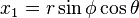
Example 1. The transformation from spherical coordinates (r, φ, θ) to Cartesian coordinates (x1, x2, x3) is given by the function F : R+ × [0,π) × [0,2π) → R3 with components:


The Jacobian matrix for this coordinate change is
![J_F(r,\phi,\theta) =\begin{bmatrix}
\dfrac{\partial x_1}{\partial r} & \dfrac{\partial x_1}{\partial \phi} & \dfrac{\partial x_1}{\partial \theta} \\[3pt]
\dfrac{\partial x_2}{\partial r} & \dfrac{\partial x_2}{\partial \phi} & \dfrac{\partial x_2}{\partial \theta} \\[3pt]
\dfrac{\partial x_3}{\partial r} & \dfrac{\partial x_3}{\partial \phi} & \dfrac{\partial x_3}{\partial \theta} \\
\end{bmatrix}=\begin{bmatrix}
\sin\phi \cos\theta & r \cos\phi \cos\theta & -r \sin\phi \sin\theta \\
\sin\phi \sin\theta & r \cos\phi \sin\theta & r \sin\phi \cos\theta \\
\cos\phi & -r \sin\phi & 0
\end{bmatrix}.](http://upload.wikimedia.org/math/7/2/6/7268ff5e31d36ed80080e6190340f03b.png)
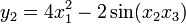
Example 2. The Jacobian matrix of the function F : R3 → R4 with components


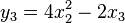

is
![J_F(x_1,x_2,x_3) =\begin{bmatrix}
\dfrac{\partial y_1}{\partial x_1} & \dfrac{\partial y_1}{\partial x_2} & \dfrac{\partial y_1}{\partial x_3} \\[3pt]
\dfrac{\partial y_2}{\partial x_1} & \dfrac{\partial y_2}{\partial x_2} & \dfrac{\partial y_2}{\partial x_3} \\[3pt]
\dfrac{\partial y_3}{\partial x_1} & \dfrac{\partial y_3}{\partial x_2} & \dfrac{\partial y_3}{\partial x_3} \\[3pt]
\dfrac{\partial y_4}{\partial x_1} & \dfrac{\partial y_4}{\partial x_2} & \dfrac{\partial y_4}{\partial x_3} \\
\end{bmatrix}=\begin{bmatrix} 1 & 0 & 0 \\ 0 & 0 & 5 \\ 0 & 8x_2 & -2 \\ x_3\cos(x_1) & 0 & \sin(x_1) \end{bmatrix}.](http://upload.wikimedia.org/math/b/4/6/b464b96f57cb3228b1c48e61be7f3d8d.png)
This example shows that the Jacobian need not be a square matrix.
[edit] In dynamical systems
Consider a dynamical system of the form x' = F(x), with F : Rn → Rn. If F(x0) = 0, then x0 is a stationary point. The behavior of the system near a stationary point can often be determined by the eigenvalues of JF(x0), the Jacobian of F at the stationary point.[1]
[edit] Jacobian determinant
If m = n, then F is a function from n-space to n-space and the Jacobian matrix is a square matrix. We can then form its determinant, known as the Jacobian determinant. The Jacobian determinant is also called the "Jacobian" in some sources.
The Jacobian determinant at a given point gives important information about the behavior of F near that point. For instance, the continuously differentiable function F is invertible near a point p ∈ Rn if the Jacobian determinant at p is non-zero. This is the inverse function theorem. Furthermore, if the Jacobian determinant at p is positive, then F preserves orientation near p; if it is negative, F reverses orientation. The absolute value of the Jacobian determinant at p gives us the factor by which the function F expands or shrinks volumes near p; this is why it occurs in the general substitution rule.
[edit] Example
The Jacobian determinant of the function F : R3 → R3 with components


is
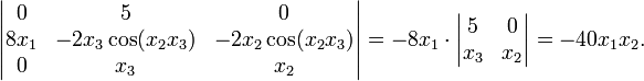
From this we see that F reverses orientation near those points where x1 and x2 have the same sign; the function is locally invertible everywhere except near points where x1 = 0 or x2 = 0. Intuitively, if you start with a tiny object around the point (1,1,1) and apply F to that object, you will get an object set with approximately 40 times the volume of the original one.
[edit] Uses
The Jacobian determinant is used when making a change of variables when integrating a function over its domain. To accommodate for the change of coordinates the Jacobian determinant arises as a multiplicative factor within the integral. Normally it is required that the change of coordinates is done in a manner which maintains an injectivity between the coordinates that determine the domain. The Jacobian determinant, as a result, is usually well defined.
[edit] See also
[edit] References
- ^ D.K. Arrowsmith and C.M. Place, Dynamical Systems, Section 3.3, Chapman & Hall, London, 1992. ISBN 0-412-39080-9.
[edit] External links
- UC Berkeley video lecture on Jacobians
- Ian Craw's Undergraduate Teaching Page An easy to understand explanation of Jacobians
- Mathworld A more technical explanation of Jacobians

