Magnetic field

From Wikipedia, the free encyclopedia

Electromagnetism

Electricity · Magnetism Electrostatics Electric charge · Coulomb's law · Electric field · Electric flux · Gauss's law · Electric potential · Electrostatic induction · Electric dipole moment · Magnetostatics Ampère’s law · Electric current · Magnetic field · Magnetic flux · Biot–Savart law · Magnetic dipole moment · Gauss’s law for magnetism · Electrodynamics Free space · Lorentz force law · EMF · Electromagnetic induction · Faraday’s law · Displacement current · Maxwell’s equations · EM field · Electromagnetic radiation · Liénard-Wiechert Potential · Maxwell tensor · Eddy current · Electrical Network Electrical conduction · Electrical resistance · Capacitance · Inductance · Impedance · Resonant cavities · Waveguides · Covariant formulation Electromagnetic tensor · EM Stress-energy tensor · Four-current · Four-potential · Scientists Ampère · Coulomb · Faraday · Heaviside · Henry · Hertz · Lorentz · Maxwell · Tesla · Weber ·

This box: view • talk • edit

Magnetic field lines shown by iron filings. The high permeability of individual iron filings causes the magnetic field to be larger at the ends of the filings. This causes individual filings to attract each other, forming elongated clusters that trace out the appearance of lines. It would not be expected that these "lines" be precisely accurate field lines for this magnet; rather, the magnetization of the iron itself would be expected to alter the field somewhat.

A magnetic field is a vector field which surrounds magnets and electric currents, and which is detected by virtue of the fact that it exerts a force on moving electric charges and on magnetic materials. When placed in a magnetic field, magnetic dipoles tend to align their axes parallel to the magnetic field. Magnetic fields also have their own energy, with an energy density proportional to the square of the field intensity.

For the physics of magnetic materials, see magnetism and magnet, and more specifically ferromagnetism, paramagnetism, and diamagnetism. For constant magnetic fields, such as are generated by magnetic materials and steady currents, see magnetostatics. A changing electric field results in a magnetic field (see electromagnetism).

The magnetic field forms one aspect of electromagnetism. (See also Classical electromagnetism and special relativity.) The electric field and magnetic field are two interrelated aspects of a single object, called the electromagnetic field, which is best known for underlying light and other electromagnetic waves. A purely electric field in one reference frame is seen as a combination of both an electric field and a magnetic field in a moving reference frame.

[edit] B and H

The term magnetic field often is used for either of two separate vector fields, denoted H and B. Although the term "magnetic field" was reserved for H in the past, today this name normally refers to B. However, modern writers do vary in their usage of B as the magnetic field.^[1] This article follows the convention of referring to the B-field and the H-field for the individual fields, and uses magnetic field where either or both fields apply.

The B-field can be defined in many equivalent ways based on the effects it has on its environment. For instance, it can be defined in terms of the force experienced by a moving charge in a magnetic field, the so-called Lorentz force (see below):

where F is the force (in newtons), B is the magnetic field (in teslas), q is the electric charge of the particle (in coulombs), v is the instantaneous velocity of the particle (in metres per second), and × is the vector cross product. A different approach to definition can be based upon a small magnet placed in a magnetic field: it will tend to twist to point in the direction of the magnetic field with a torque that is proportional to the strength of the B-field. The B-field is measured in teslas in SI units and in gauss in cgs units.

Although views have shifted over the years, B is now understood as being the fundamental quantity, while H is a derived field. So, for example, in the formulation of Maxwell's equations at a microscopic level where all charges and currents are treated explicitly, only the E- and B-fields occur. On the other hand, when charges and currents are divided into "free" and "bound" categories, D- and H-fields are used, with the H-field determined by the "free" current and time rate of change of D.^[2] Thus, when the "free" and "bound" division of currents and charges is introduced, the H-field appears and is defined as a modification of B due to material media (see magnetization, M) such that:

(definition of H )

where M is the magnetization and μ₀ is the magnetic constant.^[3] The H-field is measured in amperes per meter (A/m) in SI units and in oersteds (Oe) in cgs units.^[4]

The relationship between B and H often can be simplified for materials in which there is a simple relationship between B and M. In free space, there is no magnetization M so that H = B ⁄ μ₀ (free space). In many materials, the magnetization M is proportional to the B-field such that H = B ⁄ μ. where μ is a material dependent parameter called the permeability. In more complex materials, the permeability is a second rank tensor, which means H may not point in the same direction as B. This relation between B and H is an example of a constitutive equation. It may occur that no constitutive equation is correct, for example, in ferromagnetic materials that exhibit hysteresis the magnetization is a multiple-valued function of the B-field.^[5]

See History of B and H below for further discussion.

[edit] Alternative names for B and H

The vector field H is known among electrical engineers as the magnetic field intensity or magnetic field strength and is also known among physicists as auxiliary magnetic field or magnetizing field. The vector field B is known among electrical engineers as magnetic flux density or magnetic induction or simply magnetic field, as used by physicists.

[edit] The magnetic field and permanent magnets

The direction of the magnetic field near the poles of a magnet is revealed by placing compasses nearby. As seen here, the magnetic field points towards a magnet's south pole and away from its north pole.

Permanent magnets are objects that produce their own persistent magnetic fields. All permanent magnets have both a north and a south pole. Like poles repel and opposite poles attract. Magnetic poles always come in north-south pairs. For more details about magnets see magnetization below and the article ferromagnetism.

[edit] Force on a magnet due to a non-uniform B

The most commonly experienced effect of the magnetic field is the force between two magnets: Like poles repel and opposites attract. It is tempting, therefore, to describe the force between two magnets as a force between magnetic poles. Unfortunately, the idea of "poles" does not accurately reflect what happens inside a magnet (see ferromagnetism). Nor does this model predict the forces on a magnet due to the magnetic field that does not have poles. (For example, the magnetic field of a straight wire.)

The more physically accurate picture is that a magnet experiences a force, when placed in a non-uniform external magnetic field. The two poles of a magnet are physically separated, occupying different locations. Thus, in a nonuniform magnetic field, one pole sees a different field than the other, and consequently is subject to a different force. These two different forces can be expressed as a net force through the center of gravity plus a superposed torque. Thus, the difference in the two forces moves the magnet in the direction of increasing magnetic field. In contrast, a magnet in a uniform magnetic field experiences at most a torque, and no net magnetic force, no matter how strong the field is. The south pole of one magnet is attracted to the north pole of another because the magnetic field is not uniform, being stronger nearer to the pole.

Mathematically, the force on a magnet having a magnetic moment m is:^[6]

.

The force on a magnet due to a non-uniform magnetic field can be determined by summing up all of the forces on the elementary magnets that make up the entire magnet.

The ability of a nonuniform magnetic field to sort differently oriented dipoles is the basis of the Stern-Gerlach experiment, which established the quantum mechanical nature of the magnetic dipoles associated with atoms and electrons.^[7]

[edit] Torque on a magnet due to a B-field

A magnet placed in a magnetic field will feel a torque that will try to align the magnet with the magnetic field. The torque on a magnet due to an external magnetic field is easy to observe by placing two magnets near each other while allowing one to rotate.

The alignment of a magnet with the magnetic field of the Earth is how compasses work. It is used to determine the direction of a local magnetic field as well (see below). A small magnet is mounted such that it is free to turn (in a given plane) and its north pole is marked. By definition, the direction of the local magnetic field is the direction that the north pole of a compass (or of any magnet) tends to point.

The magnetic torque also provides the driving torque for simple electric motors. An electric motor changes electrical energy into mechanical energy (motion). In a motor, a magnet is fixed to a shaft free to rotate (forming a rotor). This magnet is subjected to a magnetic field from an array of electromagnets —called the stator. The polarity of each individual electromagnet in the stator easily can be flipped by switching the direction of the current through its coils. By flipping component electromagnet polarities in sequence, the field of the stator continuously changes to place like poles next to the rotor, subjecting the rotor to a torque that is transferred to the shaft. The inverse process, changing mechanical motion to electrical energy, is accomplished by the inverse of the above mechanism in the electric generator.

See Rotating magnetic fields below for an example using this effect with electromagnets.

[edit] Visualizing the magnetic field

Mapping out the strength and direction of the magnetic field is simple in principle. First, measure the strength and direction of the magnetic field at a large number of locations. Then mark each location with an arrow (called a vector) pointing in the direction of the local magnetic field with a length proportional to the strength of the magnetic field. An alternative method of visualizing the magnetic field which greatly simplifies the diagram while containing the same information is to 'connect' the arrows to form "magnetic field lines".

A compass placed near the north pole of a magnet will point away from that pole—like poles repel. The opposite occurs for a compass placed near a magnet's south pole. The magnetic field points away from a magnet near its north pole and towards a magnet near its south pole. Not all magnetic fields are describable in terms of poles, though. A straight current-carrying wire, for instance, produces a magnetic field that points neither towards nor away from the wire, but encircles it instead.

[edit] B-field lines

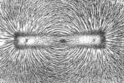
Various physical phenomena have the effect of displaying magnetic field lines. For example, iron filings placed in a magnetic field will line up in such a way as to visually show the orientation of the magnetic field (see figure at top). Another place where magnetic fields are visually displayed is in the polar auroras, in which visible streaks of light line up with the local direction of Earth's magnetic field (due to plasma particle dipole interactions). In these phenomena, lines or curves appear that follow along the direction of the local magnetic field.

These field lines provide a simple way to depict or draw the magnetic field (or any other vector field). ^[8] The magnetic field can be estimated at any point (whether on a field line or not) by looking at the direction and density of the field lines nearby.

Field lines are also a good tool for visualizing magnetic forces. When dealing with magnetic fields in ferromagnetic substances like iron, and in plasmas, the magnetic forces can be understood by imagining that the field lines exert a tension, (like a rubber band) along their length, and a pressure perpendicular to their length on neighboring field lines. The 'unlike' poles of magnets attract because they are linked by many field lines, while 'like' poles repel because the field lines between them don't meet, but run parallel, pushing on each other.

[edit] B-field lines always form loops

Field lines are a useful way to represent any vector field and often reveal sophisticated properties of fields quite simply. One important property of the B-field that can be verified with field lines is that magnetic field lines always make complete loops. Magnetic field lines neither start nor end (although they can extend to or from infinity). To date no exception to this rule has been found. (See magnetic monopole below.)

Since magnetic field lines always come in loops, magnetic poles always come in N and S pairs. Magnetic field leaves a magnet near its north pole and enters the magnet near its south pole but inside the magnet the magnetic field continues from the south pole back to the north. ^[9] If a magnetic field line enters a magnet somewhere it has to leave the magnet somewhere else; it is not allowed to have an end point. For this reason as well, cutting a magnet in half will result in two separate magnets each with both a north and a south pole.

[edit] Magnetic monopole (hypothetical)

A magnetic monopole is a hypothetical particle (or class of particles) that has, as its name suggests, only one magnetic pole (either a north pole or a south pole). In other words, it would possess a "magnetic charge" analogous to electric charge.

Modern interest in this concept stems from particle theories, notably Grand Unified Theories and superstring theories, that predict either the existence or the possibility of magnetic monopoles. These theories and others have inspired extensive efforts to search for monopoles. Despite these efforts, no magnetic monopole has been observed to date.^[10]

[edit] The magnetic field and electrical currents

Currents of electrical charges both generate a magnetic field and feel a force due to magnetic B-fields.

[edit] Electrical currents (moving charges) as a source of magnetic field

All moving charges produce a magnetic field. ^[11] The magnetic field of a moving charge is very complicated but is well known. (See Jefimenko's equations.) It forms closed loops around a line that is pointing in the direction the charge is moving. The magnetic field of a current on the other hand is much easier to calculate.

[edit] Magnetic field of a steady current

Current (I) through a wire produces a magnetic field (B) around the wire. The field is oriented according to the right hand grip rule.

The magnetic field generated by a steady current (a continual flow of charges, for example through a wire, which is constant in time and in which charge is neither building up nor depleting at any point), is described by the Biot-Savart law.^[12] This is a consequence of Ampere's law, one of the four Maxwell's equations that describe electricity and magnetism. The magnetic field lines generated by a current carrying wire form concentric circles around the wire. The direction of the magnetic field of the loops is determined by the right hand grip rule. (See figure to the right.) The strength of the magnetic field decreases with distance from the wire.

A current carrying wire can be bent in a loop such that the field is concentrated (and in the same direction) inside of the loop. The field will be weaker outside of the loop. Stacking many such loops to form a solenoid (or long coil) can greatly increase the magnetic field in the center and decrease the magnetic field outside of the solenoid. Such devices are called electromagnets and are extremely important in generating strong and well controlled magnetic fields. An infinitely long solenoid will have a uniform magnetic field inside of the loops and no magnetic field outside. A finite length electromagnet will produce essentially the same magnetic field as a uniform permanent magnet of the same shape and size. An electromagnet has the advantage, though, that you can easily vary the strength (even creating a field in the opposite direction) simply by controlling the input current. One important use is to continually switch the polarity of a stationary electromagnet to force a rotating permanent magnet to continually rotate using the fact that opposite poles attract and like poles repel. This can be used to create an important type of electrical motor.

Charged particle drifts in a homogeneous magnetic field. (A) No disturbing force (B) With an electric field, E (C) With an independent force, F (e.g. gravity) (D) In an inhomogeneous magnetic field, grad H

[edit] Force due to a B-field on a moving charge

[edit] Force on a charged particle

Beam of electrons moving in a circle. Lighting is caused by excitation of atoms of gas in a bulb.

A charged particle moving in a B-field will feel a sideways force that is proportional to the strength of the magnetic field, the component of the velocity that is perpendicular to the magnetic field and the charge of the particle. This force is known as the Lorentz force, and is given by

where

F is the force (in newtons)

q is the electric charge of the particle (in coulombs)

v is the instantaneous velocity of the particle (in meters per second)

B is the magnetic field (in teslas).

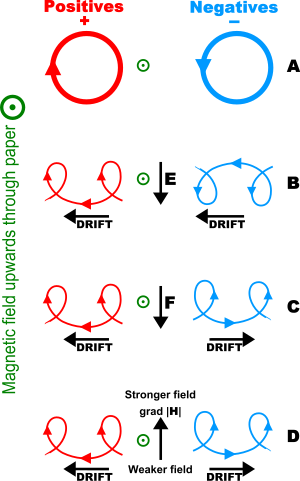
The force is always perpendicular to both the velocity of the particle and the magnetic field that created it. Neither a stationary particle nor one moving in the direction of the magnetic field lines will experience a force. For that reason, charged particles move in a circle (or more generally, in a helix) around magnetic field lines; this is called cyclotron motion. Because the magnetic field is always perpendicular to the motion, the magnetic fields can do no work on a charged particle; a magnetic field alone cannot speed up or slow down a charged particle. It can and does, however, change the particle's direction, even to the extent that a force applied in one direction can cause the particle to drift in a perpendicular direction. (See above figure.)

[edit] Force on current-carrying wire

The force on a current carrying wire is similar to that of a moving charge as expected since a charge carrying wire is a collection of moving charges. A current carrying wire will feel a sideways force in the presence of a magnetic field. The Lorentz force on a macroscopic current is often referred to as the Laplace force.

The right-hand rule: For a conventional current or moving positive charge in the direction of the thumb of the right hand and the magnetic field along the direction of the fingers (pointing away from palm) the force on the current will be in a direction out of the palm. The direction of the force is reversed for a negative charge.

[edit] Direction of force

The direction of force on a positive charge or a current is determined by the right-hand rule. See the figure on the right. Using the right hand and pointing the thumb in the direction of the moving positive charge or positive current and the fingers in the direction of the magnetic field the resulting force on the charge will point outwards from the palm. The force on a negative charged particle is in the opposite direction. If both the speed and the charge are reversed then the direction of the force remains the same. For that reason a magnetic field measurement (by itself) cannot distinguish whether there is a positive charge moving to the right or a negative charge moving to the left. (Both of these will produce the same current.) On the other hand, a magnetic field combined with an electric field can distinguish between these, see Hall effect below.

An alternative, similar trick to the right hand rule is Fleming's left hand rule.

[edit] Electromagnetism: The relationship between the magnetic and electric fields

[edit] Electric force due to a changing B-field

A magnet moving through a stationary coil will generate an electric field (and therefore a current) in the coil. This is one example of Faraday's Law which forms the basis of many electric generators. More generally, Faraday's law states that any time varying magnetic field will generate an electric field that surround the magnetic field lines in closed loops. (The generated electric field may even exist where there is no magnetic field such as outside of a long electromagnet.)

Mathematically, Faraday's law is commonly represented as:

where is the electromotive force (the voltage generated around a closed loop) and Φ_m is the magnetic flux (the product of the area times the magnetic field normal to that area). It is for this reason that engineers often refer to the B-field as the "magnetic flux density". This approach has the benefit of making certain calculations easier such as in magnetic circuits. It is typically not used outside of electrical and magnetic circuits, though, because the B-field truly is the more 'fundamental' quantity, in that it is the quantity that directly connects all of electrodynamics in the simplest manner.

In terms of the electric E and magnetic fields Faraday's Law can be written as:

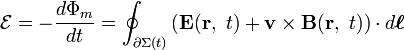
where ∂Σ(t) is the moving closed path bounding the moving surface Σ(t). In the case where the bounding surface is stationary, the Kelvin-Stokes theorem can be used to show this equation is equivalent to the Maxwell-Faraday equation:

which is one of Maxwell's equations. This equation is valid even in the presence of magnetic material.

[edit] The magnetic field due to a changing electric field

Just as a changing magnetic field generates an electric field so does a changing electric field generate a magnetic field. (These two effects bootstrap together to form electromagnetic waves, such as light.) A time varying electric field generates a magnetic field that forms closed loops around the region where the electric field is changing. The strength of this magnetic field is proportional to the time rate of the change of the electric field (which is called the displacement current). ^[13] The fact that a changing electric field creates a magnetic field is known as Maxwell's correction to Ampere's Law. Therefore the full Ampere's Law is:

where J is the current density, and partial derivatives indicate spatial location is fixed when the time derivative is taken. The last term is Maxwell's correction. This equation is always valid, but in practice it is often easier to use an alternate equation when magnetic materials are involved.

[edit] Mathematical properties of B

The magnitude of B is defined (in SI units) in terms of the voltage induced per unit area on a current carrying loop in a uniform magnetic field normal to the loop when the magnetic field is reduced to zero in a unit amount of time.

The magnetic field vector is a pseudovector (also called an axial vector). (This is a technical statement about how the magnetic field behaves when you reflect the world in a mirror.) This fact is apparent from many of the definitions and properties of the field; for example, the magnitude of the field is proportional to the torque on a dipole, and torque is a well-known pseudovector.

[edit] Maxwell's equations

As a vector field, the B-field has two important mathematical properties that relates this magnetic field to its sources. These two properties, along with the two corresponding properties of the electric field, make up Maxwell's Equations. Maxwell's Equations together with the Lorentz force law form a complete description of classical electrodynamics including both electricity and magnetism.

The first property is that a B-field line never starts nor ends at a point but instead forms a complete loop. This is mathematically equivalent to saying that the divergence of B is zero. (Such vector fields are called solenoidal vector fields.) This property is called Gauss' law for magnetism and is equivalent to the statement that there are no magnetic charges or magnetic monopoles:

where ∇ · represents the divergence operation.

The second mathematical property of the magnetic field is that it always loops around the source that creates it. This source could be a current, a magnet, or a changing electric field, but it is always within the loops of magnetic field they create. Mathematically, this fact is described by the combination of the above Gauss's law with the Ampère-Maxwell equation:

where ∇ × represents the curl operation, J = complete microscopic current density and E = electric field.

[edit] Measuring the B-field

Devices used to measure the local magnetic field are called magnetometers. Important classes of magnetometers include using a rotating coil, Hall effect magnetometers, NMR magnetometer, SQUID magnetometer, and a fluxgate magnetometer. The magnetic fields of distant astronomical objects can be determined by noting their effects on local charged particles. For instance, electrons spiraling around a field line will produce synchotron radiation which is detectable in radio waves.

[edit] Hall effect

When a current carrying conductor is placed in a transverse magnetic field the sideways Lorentz force on the charge carriers results in a charge separation in a direction perpendicular to both the current and the magnetic field. The resultant voltage, due to that charge separation, is proportional to the applied magnetic field. This is known as the Hall effect. The Hall effect is often used to measure the magnitude of a magnetic field as well as to find the sign of the dominant charge carriers in semiconductors (negative electrons or positive holes).

[edit] SQUID magnetometer

Superconductors are materials with both distinctive electric properties (perfect conductivity) and magnetic properties (such as the Meissner effect, in which many superconductors can perfectly expel magnetic fields). Due to these properties, loops of superconducting material broken up by Josephson junctions can function as very sensitive magnetometers, called SQUIDs. SQUID magnetometers are used in a Scanning SQUID microscope to create a 2D map of the magnetic field.

[edit] The magnetic field of magnetic material

[edit] Magnetic dipoles

Magnetic field lines around a ”magnetostatic dipole” the magnetic dipole itself is in the center and is seen from the side.

The magnetic field of permanent magnets and of all magnetic material originate at the atomic level. Orbiting electrons along with the nucleus form tiny magnets.^[14] The orbital component of these tiny magnets can be modeled as tiny loops of current with associated magnetic dipoles.^[15] The dipole moment of that dipole is defined as the current times the area of the loop and represents the strength of that magnet (magnetic dipole). However, in magnetic materials such as alloys of iron, cobalt and nickel, the magnetism is almost entirely spin magnetism, not orbital magnetism.^[16][17]

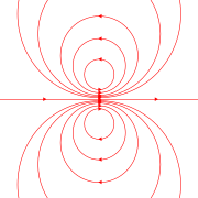
The magnetic field of an ideal magnetic dipole is depicted on the right. The magnetic field of any magnetic material is then due to the addition of the magnetic field due to the many magnetic dipoles that make up the material.

The magnetic dipole originating in an atom, electron, or nucleus is not a true dipole, as is an electric dipole. Viewing a magnetic dipole as a rotating charged sphere brings out the close connection between magnetic moment and angular momentum. Both the magnetic moment and the angular momentum increase with the rate of rotation of the sphere. The ratio of the two is called the gyromagnetic ratio, usually denoted by the symbol γ.^[18][16]

Because of the angular momentum, the dynamics of a magnetic dipole in a magnetic field differs from that of an electric dipole in an electric field. The field does exert a torque on the magnetic dipole tending to align it with the field. However, torque is proportional to rate of change of angular momentum, so precession occurs: the direction of spin changes. This behavior is described by the Landau-Lifshitz-Gilbert equation:^[19][20]

where γ =gyromagnetic ratio, m = magnetic moment, λ = damping coefficient and H_eff = effective magnetic field (the external field plus any self-field), and '×' = vector cross product. The first term describes precession of the moment about the effective field, while the second is a damping term related to dissipation of energy caused by interaction with surroundings.

[edit] Magnetization

Materials placed in a magnetic field can become magnetized. Magnetization is due to the accumulated effect of many tiny magnetic dipole moments that occur on the atomic level. In non-magnetized materials, the magnetic dipoles align randomly such that the net magnetic moment cancels producing no net magnetic field. But, if the magnetic dipoles of the material becomes aligned a net magnetization and magnetic field is produced. The magnetization field M represents how strongly a region is magnetized and is defined as the volume density of the net magnetic dipole moment in that region of material.

An equivalent way to represent magnetization is to add all of the currents of the dipole moments that produce the magnetization. The resultant current is called bound current and is the source of the magnetic field due to the magnet. Mathematically, the curl of M equals the bound current. Unlike B, though, magnetization must begin and end near the poles. (There is no magnetization outside of the material.) Therefore, the divergence of M must be non-zero near the poles of a magnet.

Most materials produce a magnetization in response to an applied B-field. Typically, the response is very weak and exists only when the magnetic field is applied. Paramagnetic materials produce a magnetization in the same direction as the applied magnetic field. Diamagnetic materials produce a magnetization that opposes the magnetic field. Ferromagnetic materials can have a magnetization independent of an applied B-field with a complex relationship between the two fields.

[edit] The H-field

The equations for the magnetic field when magnetic materials are present are simplified by introducing an 'auxiliary' H-field. The H-field is defined as:

(SI units)

(cgs units),

where M is magnetization density of any magnetic material. H is measured in amperes per meter (A/m) in SI and in oersteds (Oe) for cgs. In SI units, μ₀ is a defined constant called the magnetic constant (μ₀ = 4π × 10⁻⁷ Tm/A).

Outside of magnetizable materials the H-field differs from the B-field only by a multiplicative constant. Inside of a magnetic material they can be very different.

In many cases, the B-field is proportional to the H-field such that:

,

where μ is a material dependent parameter called the permeability. An important exception to this rule is permanent magnets. In all cases the original definitions of H in terms of B and M are still valid.

[edit] Comparison of the H- and B-fields

When a magnetic material is placed in an electromagnet, the total B-field forms closed loops around the bound current inside the magnetic material (see magnetization above) in addition to forming closed loops around the free current of the electromagnet. (Free currents are the ordinary currents in wires and other conductors, that can be directly controlled and measured.) On the other hand, the H-field forms closed loops only around free current. (Mathematically, the curl of H is equal to the free current (and the free current only) while the curl of B is proportional to the sum of both the free and the bound currents.) This simplification can in certain high symmetry cases make the calculation of the H-field much easier.

Care must be taken, though, to realize that unlike the B-field, the H-field has a portion that does not form close loops but begins and ends at something similar to 'magnetic charges'. This portion of the H-field is due to the bound currents and forms field lines that start (for both inside and outside of the magnet) near the north pole and end near the south pole. (By subtracting the magnetization from the B-field the bound current sources are converted to Gilbert-like magnetic charge distributions near the poles. More precisely, these 'magnetic charges' are calculated as −▽·M = ▽· H .)

The advantage of the hybrid H-field is that its sources are treated so differently that they can often be isolated from the other. For example, a line integral of the H-field in a closed loop will yield the total free current in the loop (not including the bound current). Similarly, a surface integral of H over any closed surface will pick out the 'magnetic charges' within that closed surface.

[edit] Uses of the H-field

[edit] Energy stored in magnetic fields

In asking how much energy does it take to create a specific magnetic field using a particular current it is important to distinguish between free and bound currents. It is the free current that we directly 'push' on to create the magnetic field. The bound currents create a magnetic field that the free current has to work against without doing any of the work.

It is not surprising, therefore, that the H-field is important in magnetic energy calculations since it treats the two sources differently. In general the incremental amount of work per unit volume δW needed to cause a small change of magnetic field δB is:

If there are no magnetic materials around then we can replace H with B ⁄ μ₀,

For linear materials (such that B = μH ), the energy density can be expressed as:

(Valid only for linear materials)

Nonlinear materials cannot use the above equation but must return to the first equation which is always valid. In particular, the energy density stored in the fields of hysteretic materials such as ferromagnets and superconductors will depend on how the magnetic field was created.

[edit] Magnetic circuits

A second use for H is in magnetic circuits where inside a linear material B = μ H. Here, μ is the magnetic permeability of the material. This result is similar in form to Ohm's Law J = σ E, where J is the current density, σ is the conductance and E is the electric field. Extending this analogy we derive the counterpart to the macroscopic Ohm's law ( I = V ⁄ R ) as:

where is the magnetic flux in the circuit, is the magnetomotive force applied to the circuit, and R_m is the reluctance of the circuit. Here the reluctance R_m is a quantity similar in nature to resistance for the flux.

Using this analogy it is straight-forward to calculate the magnetic flux of complicated magnetic field geometries, by using all the available techniques of circuit theory.

[edit] History of B and H

The modern understanding that the B-field is the more fundamental field with the H-field being an auxiliary field was not easy to arrive at. Indeed, largely because of mathematical similarities to the electric field, the H-field was developed first and was thought at first to be the more fundamental of the two. A brief history of this important transition in thought is instructional in giving insight into the nature of both H and B.

Perhaps the earliest description of a magnetic field was performed by Petrus Peregrinus and published in his “Epistola Petri Peregrini de Maricourt ad Sygerum de Foucaucourt Militem de Magnete” and is dated 1269 A.D. Petrus Peregrinus mapped out the magnetic field on the surface of a spherical magnet. Noting that the resulting field lines crossed at two points he named those points 'poles' in analogy to Earth's poles. Almost three centuries later, near the end of the sixteenth century, William Gilbert of Colchester replicated Petrus Peregrinus work and was the first to state explicitly that Earth itself was a magnet. William Gilbert's great work De Magnete was published in 1600 A.D. and helped to establish the study of magnetism as a science.

The modern distinction between the B- and H- fields does not become important until Siméon-Denis Poisson (1781–1840) developed one of the first mathematical theories of magnetism. Poisson's model, developed in 1824, assumed that magnetism was due to magnetic charges. In analogy to electric charges, these magnetic charges produce a H-field. In modern notation, Poisson's model was exactly analogous to electrostatics with the H-field replacing the electric field E-field and the B-field replacing the auxiliary D-field.

Poisson's model was, unfortunately, incorrect. Magnetism is not due to magnetic charges. Nor is magnetism created by the H-field polarizing magnetic charge in a material. The model, however, was remarkably successful for being fundamentally wrong. It predicts the correct relationship between the H-field and the B-field, even though it wrongly places H as the fundamental field with B as the auxiliary field. It predicts the correct forces between magnets.

It even predicts the correct energy stored in the magnetic fields. By the definition of magnetization, in this model, and in analogy to the physics of springs, the work done per unit volume, in stretching and twisting the bonds between magnetic charge to increment the magnetization by μ₀δM is W = H · μ₀δM. In this model, B = μ₀ (H + M ) is an effective magnetization which includes the H-field term to account for the energy of setting up the magnetic field in a vacuum. Therefore the total energy density increment needed to increment the magnetic field is W = H · δB. This is the correct result, but it is derived from an incorrect model.

In retrospect the success of this model is due largely to the remarkable coincidence that from the 'outside' the field of an electric dipole has the exact same form as that of a magnetic dipole. It is therefore only for the physics of magnetism 'inside' of magnetic material where the simpler model of magnetic charges fails. It is also important to note that this model is still useful in many situations dealing with magnetic material. One example of its utility is the concept of magnetic circuits.

The formation of the correct theory of magnetism begins with a series of revolutionary discoveries in 1820, four years before Poisson's model was developed. (The first clue that something was amiss, though, was that unlike electrical charges magnetic poles cannot be separated from each other or form magnetic currents.) The revolution began when Hans Christian Oersted discovered that an electrical current generates a magnetic field that encircles the wire. In a quick succession that discovery was followed by Andre Marie Ampere showing that parallel wires having currents in the same direction attract, and by Jean-Baptiste Biot and Felix Savart developing the correct equation, the Biot-Savart Law, for the magnetic field of a current carrying wire. In 1825, Ampere extended this revolution by publishing his Ampere's Law which provided a more mathematically subtle and correct description of the magnetic field generated by a current than the Biot-Savart Law.

Subsequent development in the nineteenth century interlinked magnetic and electric phenomena even tighter, until the concept of magnetic charge was not needed. Magnetism became an electric phenomenon with even the magnetism of permanent magnets being due to small loops of current in their interior. This development was aided greatly by Michael Faraday, who in 1831 showed that a changing magnetic field generates an encircling electric field. The final blow to magnetic charge was delivered by James Clerk Maxwell in a series of three great works that established Maxwell's equations which formed a complete foundation of classical electrodynamics. Maxwell's equations have only two sources for the electric and magnetic fields: electric charge, and electric current. Though the original source for the H-field was rejected, the H-field still had a prominent role in Maxwell's equations. But, now it was as an auxiliary field to the fundamental B-field.

Although the classical theory of electrodynamics was essentially complete with Maxwell's equations, the twentieth century saw a number of improvements and extensions to the theory. Albert Einstein in his great paper of 1905 that established relativity, showed that both the electric and magnetic fields were part of the same phenomena viewed from different reference frames. Finally, the emergent field of quantum mechanics was merged with electrodynamics to form quantum electrodynamics or QED.

[edit] Special relativity and electromagnetism

Magnetic fields played an important role in helping to develop the theory of special relativity.

[edit] Moving magnet and conductor problem

Imagine a moving conducting loop that is passing by a stationary magnet. Such a conducting loop will have a current generated in it as it passes through the magnetic field. But why? It is answering this seemingly innocent question that led Albert Einstein to develop his theory of special relativity.

A stationary observer would see an unchanging magnetic field and a moving conducting loop. Since the loop is moving all of the charges that make up the loop are also moving. Each of these charges will have a sideways, Lorentz force, acting on it which generates the current. Meanwhile, an observer on the moving reference frame would see a changing magnetic field and stationary charges. (The loop is not moving in this observers reference frame. The magnet is.) This changing magnetic field generates an electric field.

The stationary observer claims there is only a magnetic field that creates a magnetic force on a moving charge. The moving observer claims that there is both a magnetic and an electric field but all of the force is due to the electric field. Which is true? Does the electric field exist or not? The answer, according to special relativity, is that both observers are right from their reference frame. A pure magnetic field in one reference can be a mixture of magnetic and electric field in another reference frame.

[edit] Electric and magnetic fields different aspects of the same phenomenon

According to special relativity, electric and magnetic forces are part of a single physical phenomenon, electromagnetism; an electric force perceived by one observer will be perceived by another observer in a different frame of reference as a mixture of electric and magnetic forces. Magnetic and electric forces are facets of the underlying electromagnetic force, and the partition of the electromagnetic force into separate electric and magnetic components is not fundamental, but varies with the observational frame of reference.

More specifically, rather than treating the electric and magnetic fields as separate fields, special relativity shows that they naturally mix together into a rank-2 tensor, called the electromagnetic tensor. This is analogous to the way that special relativity "mixes" space and time into spacetime, and mass, momentum and energy into four-momentum.

[edit] Magnetic field shape descriptions

Schematic quadrupole magnet ("four-pole") magnetic field. There are four steel pole tips, two opposing magnetic north poles and two opposing magnetic south poles.

• An azimuthal magnetic field is one that runs east-west.

• A meridional magnetic field is one that runs north-south. In the solar dynamo model of the Sun, differential rotation of the solar plasma causes the meridional magnetic field to stretch into an azimuthal magnetic field, a process called the omega-effect. The reverse process is called the alpha-effect.^[21]

• A dipole magnetic field is one seen around a bar magnet or around a charged elementary particle with nonzero spin.

• A quadrupole magnetic field is one seen, for example, between the poles of four bar magnets. The field strength grows linearly with the radial distance from its longitudinal axis.

• A solenoidal magnetic field is similar to a dipole magnetic field, except that a solid bar magnet is replaced by a hollow electromagnetic coil magnet.

• A toroidal magnetic field occurs in a doughnut-shaped coil, the electric current spiraling around the tube-like surface, and is found, for example, in a tokamak.

• A poloidal magnetic field is generated by a current flowing in a ring, and is found, for example, in a tokamak.

• A radial magnetic field is one in which the field lines are directed from the center outwards, similar to the spokes in a bicycle wheel. An example can be found in a loudspeaker transducers (driver).^[22]

• A helical magnetic field is corkscrew-shaped, and sometimes seen in space plasmas such as the Orion Molecular Cloud.^[23]

[edit] Important uses and examples of magnetic field

[edit] Earth's magnetic field

A sketch of Earth's magnetic field representing the source of Earth's magnetic field as a magnet. The north pole of earth is near the top of the diagram, the south pole near the bottom. Notice that the south pole of that magnet is deep in Earth's interior below Earth's North Magnetic Pole. Earth's magnetic field is produced in the outer liquid part of its core due to a dynamo that produce electrical currents there.

Because of Earth's magnetic field, a compass placed anywhere on Earth will turn so that the "north pole" of the magnet inside the compass points roughly north, toward Earth's north magnetic pole in northern Canada. This is the traditional definition of the "north pole" of a magnet, although other equivalent definitions are also possible. One confusion that arises from this definition is that if Earth itself is considered as a magnet, the south pole of that magnet would be the one nearer the north magnetic pole, and vice-versa. (Opposite poles attract and the north pole of the compass magnet is attracted to the north magnetic pole.) The north magnetic pole is so named not because of the polarity of the field there but because of its geographical location.

The figure to the right is a sketch of Earth's magnetic field represented by field lines. The magnetic field at any given point does not point straight toward (or away) from the poles and has a significant up/down component for most locations. (In addition, there is an East/West component as Earth's magnetic poles do not coincide exactly with Earth's geological pole.) The magnetic field is as if there were a magnet deep in Earth's interior.

Earth's magnetic field is probably due to a dynamo that produces electric currents in the outer liquid part of its core. Earth's magnetic field is not constant: Its strength and the location of its poles vary. The poles even periodically reverse direction, in a process called geomagnetic reversal.

[edit] Rotating magnetic fields

The rotating magnetic field is a key principle in the operation of alternating-current motors. A permanent magnet in such a field will rotate so as to maintain its alignment with the external field. This effect was conceptualized by Nikola Tesla, and later utilized in his, and others', early AC (alternating-current) electric motors. A rotating magnetic field can be constructed using two orthogonal coils with 90 degrees phase difference in their AC currents. However, in practice such a system would be supplied through a three-wire arrangement with unequal currents. This inequality would cause serious problems in standardization of the conductor size and so, in order to overcome it, three-phase systems are used where the three currents are equal in magnitude and have 120 degrees phase difference. Three similar coils having mutual geometrical angles of 120 degrees will create the rotating magnetic field in this case. The ability of the three-phase system to create a rotating field, utilized in electric motors, is one of the main reasons why three-phase systems dominate the world's electrical power supply systems.

Because magnets degrade with time, synchronous motors and induction motors use short-circuited rotors (instead of a magnet) following the rotating magnetic field of a multicoiled stator. The short-circuited turns of the rotor develop eddy currents in the rotating field of the stator, and these currents in turn move the rotor by the Lorentz force.

In 1882, Nikola Tesla identified the concept of the rotating magnetic field. In 1885, Galileo Ferraris independently researched the concept. In 1888, Tesla gained U.S. Patent 381,968  for his work. Also in 1888, Ferraris published his research in a paper to the Royal Academy of Sciences in Turin.

[edit] See also

General

• Electric field — field produced by electric charges and changing magnetic fields that affects charged particles.
• Electromagnetic field — a field composed of the electric field and the magnetic field.
• Electromagnetism — the physics of the electromagnetic field.
• Faraday's law of induction — the connection between electric and magnetic fields as found in motors and generators
• Lorentz force — the connection between fields and forces
• Magnetism — phenomenon by which materials exert a magnetic force on other materials.
• Magnetohydrodynamics — the study of the dynamics of electrically conducting fluids.
• Magnetic flux — amount of 'magnetic field' through a given loop.
• Magnetic monopole — hypothetical particle which causes nonzero divergence of magnetic field.
• Magnetic nanoparticles — extremely small magnetic particles that are tens of atoms wide
• Magnetic reconnection — an effect which causes solar flares and auroras.
• Magnetic potential — the vector and scalar potential representation of magnetism.
• SI electromagnetism units — common units used in electromagnetism.
• Orders of magnitude (magnetic field) — list of magnetic field sources and measurement devices from smallest magnetic fields to largest detected.

Mathematics

• Ampère's law — law describing how currents act as circulation sources for magnetic fields.
• Biot-Savart law — the magnetic field set up by a steadily flowing line current.
• Magnetic helicity — extent to which a magnetic field "wraps around itself".
• Maxwell's equations — four equations describing the behavior of electric and magnetic fields and their interaction with matter.

Applications

• Dynamo theory — a proposed mechanism for the creation of the Earth's magnetic field.
• Earth's magnetic field — a discussion of the magnetic field of the Earth.
• Electric motor — AC motors used magnetic fields.
• Helmholtz coil — a device for producing a region of nearly uniform magnetic field.
• Magnetic field viewing film — Film used to view the magnetic field of an area.
• Maxwell coil — a device for producing a large volume of almost constant magnetic field.
• Stellar magnetic field — a discussion of the magnetic field of stars.
• Teltron Tube — device used to display an electron beam and demonstrates effect of electric and magnetic fields on moving charges.

[edit] Further reading

[edit] Notes and references

[edit] External links

Information

• Crowell, B., "Electromagnetism".

• Nave, R., "Magnetic Field". HyperPhysics.

• "Magnetism", The Magnetic Field. theory.uwinnipeg.ca.

• Hoadley, Rick, "What do magnetic fields look like?" 17 July 2005.

Field density

• Jiles, David (1994). Introduction to Electronic Properties of Materials (1st ed.). Springer. ISBN 0-412-49580-5.

Rotating magnetic fields

• "Rotating magnetic fields". Integrated Publishing.

• "Introduction to Generators and Motors", rotating magnetic field. Integrated Publishing.

• "Induction Motor-Rotating Fields".

Diagrams

• McCulloch, Malcolm,"A2: Electrical Power and Machines", Rotating magnetic field. eng.ox.ac.uk.

• "AC Motor Theory" Figure 2 Rotating Magnetic Field. Integrated Publishing.

Journal Articles

• Yaakov Kraftmakher, "Two experiments with rotating magnetic field". 2001 Eur. J. Phys. 22 477-482.

• Bogdan Mielnik and David J. Fernández C., "An electron trapped in a rotating magnetic field". Journal of Mathematical Physics, February 1989, Volume 30, Issue 2, pp. 537-549.

• Sonia Melle, Miguel A. Rubio and Gerald G. Fuller "Structure and dynamics of magnetorheological fluids in rotating magnetic fields". Phys. Rev. E 61, 4111 – 4117 (2000).