RLC circuit

Linear analog electronic filters
	Network synthesis filters Image impedance filters Simple filters RL filter; RC filter; RLC filter; LC filter;
	edit

From Wikipedia, the free encyclopedia

Jump to: navigation, search

An RLC circuit (also known as a resonant circuit, tuned circuit, or LCR circuit) is an electrical circuit consisting of a resistor (R), an inductor (L), and a capacitor (C), connected in series or in parallel. This configuration forms a harmonic oscillator.

Tuned circuits have many applications particularly for oscillating circuits and in radio and communication engineering. They can be used to select a certain narrow range of frequencies from the total spectrum of ambient radio waves. For example, AM/FM radios with analog tuners typically use an RLC circuit to tune a radio frequency. Most commonly a variable capacitor is attached to the tuning knob, which allows you to change the value of C in the circuit and tune to stations on different frequencies.

An RLC circuit is called a second-order circuit as any voltage or current in the circuit can be described by a second-order differential equation for circuit analysis.

1 Configurations
2 Similarities and differences between series and parallel circuits
3 Fundamental parameters
4 Derived parameters
- 4.1 Bandwidth
- 4.2 Damped resonance
5 Circuit analysis
- 5.1 Series RLC with Thévenin power source
  - 5.1.1 Frequency domain
- 5.2 Parallel RLC circuit
6 See also
7 External links

[edit] Configurations

Every RLC circuit consists of two components: a power source and resonator. There are two types of power sources – Thévenin and Norton. Likewise, there are two types of resonators – series LC and parallel LC. As a result, there are four configurations of RLC circuits:

Series LC with Thévenin power source
Series LC with Norton power source
Parallel LC with Thévenin power source
Parallel LC with Norton power source.

It is relatively easy to show that each of the two series configurations can be transformed into the other using elementary network transformations – specifically, by transforming the Thévenin power source to the equivalent Norton power source, or vice versa. Likewise, each of the two parallel configurations can be transformed into the other using the same network transformations. Finally, the Series/Thévenin and the Parallel/Norton configurations are dual circuits of one another. Likewise, the Series/Norton and the Parallel/Thévenin configurations are also dual circuits.

[edit] Similarities and differences between series and parallel circuits

The expressions for the bandwidth in the series and parallel configuration are inverses of each other. This is particularly useful for determining whether a series or parallel configuration is to be used for a particular circuit design. However, in circuit analysis, usually the reciprocal of the latter two variables is used to characterize the system instead. They are known as the resonant frequency and the Q factor respectively.

[edit] Fundamental parameters

There are two fundamental parameters that describe the behavior of RLC circuits: the resonant frequency and the attenuation (or, alternatively, the damping factor). In addition, other parameters derived from these first two are discussed below.

[edit] Resonant frequency

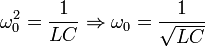
The undamped resonant frequency of an RLC circuit (in radians per second) is given by

$\omega_0 = {1 \over \sqrt{L C}}$

In the more familiar unit hertz (or cycles per second), the resonant frequency becomes

$f_0 = {\omega_0 \over 2 \pi} = {1 \over 2 \pi \sqrt{L C}}$

Resonance occurs when the complex impedance Z_LC of the LC resonator becomes zero:

$Z_{LC} = Z_L + Z_C = 0\quad$

Both of these impedances are functions of angular frequency $ω$ :

$Z_C = {1 \over {j \omega C}}$

$Z_L = jL\omega \quad$

Setting the magnitude of the impedance to be zero at $ω = ω 0$ and using $j 2 = - 1$ :

$|Z_{LC}|=L\omega_0-{1\over {\omega_0 C}}=0$

$\omega_0^2={1\over{LC}}\Rightarrow\omega_0={1\over\sqrt{LC}}$

[edit] Attenuation

The attenuation α is defined as

$\alpha = {R \over 2L }$

for the series RLC circuit, and

$\alpha = {1 \over 2RC }$

for the parallel RLC circuit.

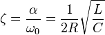
[edit] Damping factor

The damping factor ζ is the ratio of the attenuation α to the resonant frequency ω₀ :

$\zeta = {\alpha \over\omega_0} = {R \over 2} \sqrt{C\over L}$

for a series RLC circuit, and:

$\zeta = {\alpha \over\omega_0} = {1 \over 2R}\sqrt{L\over C}$

for a parallel RLC circuit.

It is sometimes more convenient to use the damping factor, which is dimensionless, instead of the attenuation factor, which has dimensions of radians per second, to analyze the properties of a resonant circuit.

[edit] Minimizing the attenuation for oscillator circuits

For applications in oscillator circuits, it is generally desirable to make the attenuation (or equivalently, the damping factor) as small as possible. In practice, this objective requires making the circuit's resistance R as small as physically possible for a series circuit, or alternatively increasing R to as much as as possible for a parallel circuit. In either case, the RLC circuit becomes a good approximation to an ideal LC circuit.

Alternatively, for applications in bandpass filters, the value of the damping factor is chosen based on the desired bandwidth of the filter. For a wider bandwidth, a larger value of the damping factor is required (and vice versa). In practice, this requires adjusting the relative values of the resistor R and the inductor L in the circuit.

[edit] Derived parameters

The derived parameters include bandwidth, Q factor, and damped resonance frequency.

[edit] Bandwidth

The RLC circuit may be used as a bandpass or band-stop filter by replacing R with a receiving device with the same input resistance. In the Series case the bandwidth (in radians per second) is

$\Delta \omega = 2 \alpha = 2 \zeta \omega_0 = { R \over L}$

Alternatively, the bandwidth in hertz is

$\Delta f = { \Delta \omega \over 2 \pi } = { \alpha \over \pi } = { \zeta \omega_0 \over \pi } = { R \over 2 \pi L }$

The bandwidth is a measure of the width of the frequency response at the two half-power frequencies. As a result, this measure of bandwidth is sometimes called the full-width at half-power. Since electrical power is proportional to the square of the circuit voltage (or current), the frequency response will drop to ${ 1 \over \sqrt{2} }$ at the half-power frequencies.

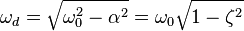
[edit] Damped resonance

The damped resonance frequency can be expressed in terms of the undamped resonance frequency and the damping factor. If the circuit is underdamped, meaning

$\displaystyle \alpha < \omega_0$

or equivalently

$\displaystyle \zeta < 1$

then we can define the damped resonance as

$\omega_d = \sqrt{ \omega_0^2 - \alpha^2 } = \omega_0 \sqrt{ 1 - \zeta^2 }$

In an oscillator circuit

$\alpha \ll \omega_0$ .

or equivalently

$\zeta \ll 1$ .

As a result

$\omega_d \approx \omega_0$ .

See discussion of underdamping, overdamping, and critical damping, below.

[edit] Circuit analysis

[edit] Series RLC with Thévenin power source

In this circuit, the three components are all in series with the voltage source.

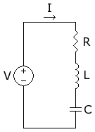Series RLC Circuit notations:

V - the voltage of the power source (measured in volts V)

I - the current in the circuit (measured in amperes A)

R - the resistance of the resistor (measured in ohms = V/A);

L - the inductance of the inductor (measured in henrys = H = V·s/A)

C - the capacitance of the capacitor (measured in farads = F = C/V = A·s/V)

q - the charge across the capacitor (measured in coulombs C)

Given the parameters v, R, L, and C, the solution for the charge, q, can be found using Kirchhoff's voltage law. (KVL) gives

${v_R+v_L+v_C=v} \,$

For a time-changing voltage v(t), this becomes

$Ri(t) + L { {di} \over {dt}} + {1 \over C} \int_{-\infty}^{t} i(\tau)\, d\tau = v(t)$

Using the relationship between charge and current:

$i(t) = {{dq} \over {dt}}$

The above expression can be expressed in terms of charge across the capacitor:

$L {{d^2 q} \over {dt^2}} +{R} {{dq} \over {dt}} + {1 \over {C}} q(t) = v(t)$

Dividing by L gives the following second order differential equation:

${{d^2 q} \over {dt^2}} +{R \over L} {{dq} \over {dt}} + {1 \over {LC}} q(t) = {1 \over L} v(t)$

We now define two key parameters:

$\zeta_N = {R \over 2} \sqrt{C \over L}$ and $\omega_0 = { 1 \over \sqrt{LC}}$

Substituting these parameters into the differential equation, we obtain:

${{d^2 q} \over {dt^2}} + 2 \zeta_N . \omega_0{{dq} \over {dt}} + \omega_0^2 q(t) = {1 \over L} v(t)$

or

$\ddot{q}+2\zeta_N . \omega_0 \dot{q} + \omega_0^2 q = {1 \over L} v(t)$

[edit] Frequency domain

The series RLC can be analyzed in the frequency domain using complex impedance relations. If the voltage source above produces a complex exponential waveform with complex amplitude V(s) and angular frequency $s = σ + i ω$ , KVL can be applied:

$V(s) = I(s) \left ( R + Ls + \frac{1}{Cs} \right )$

where I(s) is the complex current through all components. Solving for I(s):

$I(s) = \frac{1}{ R + Ls + \frac{1}{Cs} } V(s)$

And rearranging, we have at

$I(s) = \frac{s}{ L \left ( s^2 + {R \over L}s + \frac{1}{LC} \right ) } V(s)$

[edit] Complex admittance

Next, we solve for the complex admittance Y(s):

$Y(s) = { I(s) \over V(s) } = \frac{s}{ L \left ( s^2 + {R \over L}s + \frac{1}{LC} \right ) }$

Finally, we simplify using parameters α and ω_o

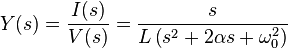
$Y(s) = { I(s) \over V(s) } = \frac{s}{ L \left ( s^2 + 2 \alpha s + \omega_0^2 \right ) }$

Notice that this expression for Y(s) is the same as the one we found for the Zero State Response.

[edit] Poles and zeros

The zeros of Y(s) are those values of s such that $Y (s) = 0$ :

$s = 0 \,$ and $|s| \rightarrow \infty$

The poles of Y(s) are those values of s such that $Y(s) \rightarrow \infty$ . By the quadratic formula, we find

$s = - \alpha \pm \sqrt{\alpha^2 - \omega_0^2}$

Notice that the poles of Y(s) are identical to the roots $λ 1$ and $λ 2$ of the characteristic polynomial.

[edit] Sinusoidal steady state

If we now let $s = i ω$ ....

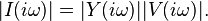
Taking the magnitude of the above equation:

$| Y(s=i \omega) | = \frac{1}{\sqrt{ R^2 + \left ( \omega L - \frac{1}{\omega C} \right )^2 }}.$

Next, we find the magnitude of current as a function of ω

$| I( i \omega ) | = | Y(i \omega) | | V(i \omega) |.\,$

If we choose values where R = 1 ohm, C = 1 farad, L = 1 henry, and V = 1.0 volt, then the graph of magnitude of the current i (in amperes) as a function of ω (in radians per second) is:

Sinusoidal steady-state analysis

Note that there is a peak at $i m a g (ω) = 1$ . This is known as the resonant frequency. Solving for this value, we find:

$\omega_0 = \frac{1}{\sqrt{L C}}.$

[edit] Parallel RLC circuit

Parallel RLC Circuit notations:

V - the voltage of the power source (measured in volts V)

I - the current in the circuit (measured in amperes A)

R - the resistance of the resistor (measured in ohms = V/A);

L - the inductance of the inductor (measured in henrys = H = V·s/A)

C - the capacitance of the capacitor (measured in farads = F = C/V = A·s/V)

The complex admittance of this circuit is given by adding up the admittances of the components:

${1\over Z}={1\over Z_L}+{1\over Z_C}+{1\over Z_R}={1\over{j\omega L}}+{j\omega C}+{1\over R}$

The change from a series arrangement to a parallel arrangement has some very real consequences for the behaviour. This can be seen by plotting the magnitude of the current $I={V\over Z}$ . For comparison with the earlier graph we choose values where R = 1 ohm, C = 1 farad, L = 1 henry, and V = 1.0 volt and ω in radians per second:

Sinusoidal steady-state analysis

There is a minimum in the frequency response at the resonant frequency $\omega_0={1\over\sqrt{LC}}$ .

A parallel RLC circuit is a example of a band-stop circuit response that can be used as a filter to block frequencies at the resonance frequency but allow others to pass.

[edit] See also

[edit] External links