Fourier transform
From Wikipedia, the free encyclopedia
In mathematics, the Fourier transform is an operation that transforms one complex-valued function of a real variable into another. The new function, often called the frequency domain representation of the original function, describes which frequencies are present in the original function. This is in a similar spirit to the way that a chord of music can be described by notes that are being played. In effect, the Fourier transform decomposes a function into oscillatory functions. The Fourier transform (FT) is similar to many other operations in mathematics which make up the subject of Fourier analysis. In this specific case, both the domains of the original function and its frequency domain representation are continuous and unbounded. The term Fourier transform can refer to both the frequency domain representation of a function or to the process/formula that "transforms" one function into the other.
| Fourier transforms |
|---|
| Continuous Fourier transform |
| Fourier series |
| Discrete Fourier transform |
| Discrete-time Fourier transform |
|
|
Contents |
[edit] Definition
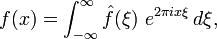
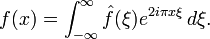
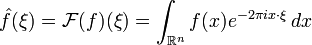
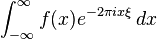
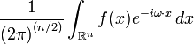
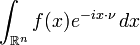
There are several common conventions for defining the Fourier transform of an integrable function ƒ : R → C (Kaiser 1994). This article will use the definition:
 for every real number ξ. (This letter is the lowercase Greek letter Xi).
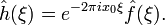
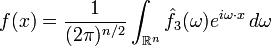
When the independent variable x represents time (with SI unit of seconds), the transform variable ξ represents ordinary frequency (in hertz). Under suitable conditions, ƒ can be reconstructed from  by the inverse transform:
 for every real number x.
For other common conventions and notations see the sections Other conventions and Other notations below.
[edit] Introduction
The motivation for the Fourier transform comes from the study of Fourier series. In the study of Fourier series, complicated periodic functions are written as the sum of simple waves mathematically represented by sines and cosines. Due to the properties of sine and cosine it is possible to recover the amount of each wave in the sum by an integral. In many cases it is desirable to use Euler's formula, which states that e2πiθ = cos 2πθ + i sin 2πθ, to write Fourier series in terms of the basic waves e2πiθ. This has the advantage of simplifying many of the formulas involved and providing a formulation for Fourier series that more closely resembles the definition followed in this article. This passage from sines and cosines to complex exponentials makes it necessary for the Fourier coefficients to be complex valued. The usual interpretation of this complex number is that it gives you both the amplitude (or size) of the wave present in the function and the phase (or the initial angle) of the wave. This passage also introduces the need for negative "frequencies". If θ were measured in seconds then the waves e2πiθ and e−2πiθ would both complete one cycle per second, but they represent different frequencies in the Fourier transform. Hence, frequency no longer measures the number of cycles per unit time, but is closely related.
We may use Fourier series to motivate the Fourier transform as follows. Suppose that ƒ is a function which is zero outside of some interval [−L/2, L/2]. Then for any T ≥ L we may expand ƒ in a Fourier series on the interval [−T/2,T/2], where the "amount" (denoted by cn) of the wave e2πinx/T in the Fourier series of ƒ is given by

and ƒ should be given by the formula

If we let ξn = n/T, and we let Δξ = (n + 1)/T − n/T = 1/T, then this last sum becomes the Riemann sum

By letting T → ∞ this Riemann sum converges to the integral for the inverse Fourier transform given in the Definition section. Under suitable conditions this argument may be made precise (Stein & Shakarchi 2003). Hence, as in the case is Fourier series, the Fourier transform can be thought of as a function that measures how much of each individual frequency is present in our function, and we can recombine these waves by using an integral (or "continuous sum") to reproduce the original function.
The following images provide a visual illustration of how the Fourier transform measures whether a frequency is present in a particular function. The function depicted 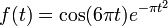 oscillates at 3 hertz (if t measures seconds) and tends quickly to 0. This function was specially chosen to have a real Fourier transform which can easily be plotted. The first image contains its graph. In order to calculate
  we must integrate e−2πi(3t)ƒ(t). The second image shows the plot of the real and imaginary parts of this function. The real part of the integrand is almost always positive, this is because when ƒ(t) is negative, then the real part of e−2πi(3t) is negative as well. Because they oscillate at the same rate, when ƒ(t) is positive, so is the real part of e−2πi(3t). The result is that when you integrate the real part of the integrand you get a relatively large number (in this case 0.5). On the other hand, when you try to measure a frequency that is not present, as in the case when we look at
  , the integrand oscillates enough so that the integral is very small. The general situation may be a bit more complicated than this, but this in spirit is how the Fourier transform measures how much of an individual frequency is present in a function ƒ(t).
 Original function showing oscillation 3 hertz. |
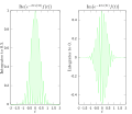 Real and imaginary parts of integrand for Fourier transform at 3 hertz |
 Real and imaginary parts of integrand for Fourier transform at 5 hertz |
Fourier transform with 3 and 5 hertz labeled. |
[edit] Properties of the Fourier transform
An integrable function is a function ƒ on the real line that is Lebesgue-measurable and satisfies

[edit] Basic properties
Given integrable functions f(x), g(x), and h(x) denote their Fourier transforms by  ,
,  , and
, and  respectively. The Fourier transform has the following basic properties (Pinsky 2002).
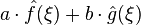
- Linearity
- For any complex numbers a and b, if h(x) = aƒ(x) + bg(x), then

- Translation
- For any real number x0, if h(x) = ƒ(x − x0), then
- Modulation
- For any real number ξ0, if h(x) = e2πixξ0ƒ(x), then
 .
. - Scaling
- For all non-zero real numbers a, if h(x) = ƒ(ax), then
 . The case a = −1 leads to the time-reversal property, which states: if h(x) = ƒ(−x), then
  .
. - Conjugation
- If
 , then
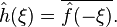
- Convolution
- If
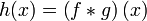 , then
[edit] Uniform continuity and the Riemann-Lebesgue lemma
The Fourier transform of integrable functions have additional properties that do not always hold. The Fourier transform of integrable functions ƒ are uniformly continuous and  (Katznelson 1976). The Fourier transform of integrable functions also satisfy the Riemann-Lebesgue lemma which states that (Stein & Weiss 1971)

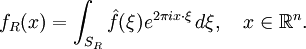
The Fourier transform of an integrable function ƒ is bounded and continuous, but need not be integrable. It is not possible in general to write the inverse transform as a Lebesgue integral. However, when both ƒ and are integrable, the following inverse equality holds true for almost every x:
Almost everywhere, ƒ is equal to the continuous function given by the right-hand side. If ƒ is given as continuous function on the line, then equality holds for every x.
A consequence of the preceding result is that the Fourier transform is injective on L1(R).
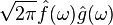
[edit] The Plancherel theorem and Parseval's theorem
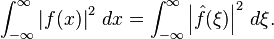
Let f(x) and g(x) be integrable, and let and be their Fourier transforms. If f(x) and g(x) are also square-integrable, then we have Parseval's theorem (Rudin 1987, p. 187):

where the bar denotes complex conjugation.
The Plancherel theorem, which is equivalent to Parseval's theorem, states (Rudin 1987, p. 186):
The Plancherel theorem makes it possible to define the Fourier transform for functions in L2(R), as described in Generalizations below. The Plancherel theorem has the interpretation in the sciences that the Fourier transform preserves the energy of the original quantity. It should be noted that depending on the author either of these theorems might be referred to as the Plancherel theorem or as Parseval's theorem.
See Pontryagin duality for a general formulation of this concept in the context of locally compact abelian groups.
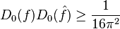
[edit] Uncertainty principle
Generally speaking, the more concentrated f(x) is, the more spread out its Fourier transform must be. In particular, the scaling property of the Fourier transform may be seen as saying: if we "squeeze" a function in x, its Fourier transform "stretches out" in ξ. It is not possible to arbitrarily concentrate both a function and its Fourier transform.
The trade-off between the compaction of a function and its Fourier transform can be formalized in the form of an Uncertainty Principle. Suppose ƒ(x) is an integrable and square-integrable function. Without loss of generality, assume that ƒ(x) is normalized:

It follows from the Plancherel theorem that is also normalized.
The spread around x = 0 may be measured by the dispersion about zero (Pinsky 2002) defined by

In probability terms, this is the second moment of  about zero.
The Uncertainty principle states that, if ƒ(x) is absolutely continuous and the functions x·ƒ(x) and ƒ′(x) are square integrable, then
 (Pinsky 2002).
The equality is attained only in the case  (hence
 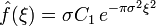 ) where σ > 0 is arbitrary and C1 is such that ƒ is L2–normalized (Pinsky 2002). In other words, where ƒ is a (normalized) Gaussian function, centered at zero.
In fact, this inequality implies that:

for any  in R (Stein & Shakarchi 2003).
In quantum mechanics, the momentum and position wave functions are Fourier transform pairs, to within a factor of Planck's constant. With this constant properly taken into account, the inequality above becomes the statement of the Heisenberg uncertainty principle (Stein & Shakarchi 2003).
[edit] Poisson summation formula
The Poisson summation formula provides a link between the study of Fourier transforms and Fourier Series. Given an integrable function ƒ in L1(Rn) we can consider the periodization of ƒ given by
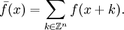
Then the Poisson summation formula relates the Fourier series of  to the Fourier transform of ƒ. Specifically it states that the Fourier series of is given by:
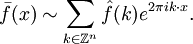
The Poisson summation formula maybe used to derive Landau's asymptotic formula for the number of lattice points in a large Euclidean sphere. It can also be used to show that if an integrable function, ƒ, and both have compact support then ƒ = 0 (Pinsky 2002).
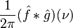
[edit] Convolution theorem
The Fourier transform translates between convolution and multiplication of functions. If ƒ(x) and g(x) are integrable functions with Fourier transforms and respectively, and if the convolution of ƒ and g exists and is absolutely integrable, then the Fourier transform of the convolution is given by the product of the Fourier transforms and (under other conventions for the definition of the Fourier transform a constant factor may appear).
This means that if:
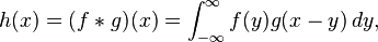
where ∗ denotes the convolution operation, then:
In linear time invariant (LTI) system theory, it is common to interpret g(x) as the impulse response of an LTI system with input ƒ(x) and output h(x), since substituting the unit impulse for ƒ(x) yields h(x) = g(x). In this case, represents the frequency response of the system.
Conversely, if ƒ(x) can be decomposed as the product of two square integrable functions p(x) and q(x), then the Fourier transform of ƒ(x) is given by the convolution of the respective Fourier transforms  and
and  .
.
[edit] Cross-correlation theorem
In an analogous manner, it can be shown that if h(x) is the cross-correlation of ƒ(x) and g(x):

then the Fourier transform of h(x) is:

[edit] Eigenfunctions
One important choice of an orthonormal basis for L2(R) is given by the Hermite functions
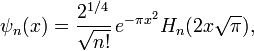
where Hn(x) are the "probabilist's" Hermite polynomials, defined by Hn(x) = (−1)nexp(x2/2) Dn exp(−x2/2). Under this convention for the Fourier transform, we have that

In other words, the Hermite functions form a complete orthonormal system of eigenfunctions for the Fourier transform on L2(R) (Pinsky 2002). However, this choice of eigenfunctions is not unique. There are only four different eigenvalues of the Fourier transform (±1 and ±i) and any linear combination of eigenfunctions with the same eigenvalue gives another eigenfunction. As a consequence of this, it is possible to decompose L2(R) as a direct sum of four spaces H0, H1, H2, and H3 where the Fourier transform acts on Hk simply by multiplication by ik. This approach to define the Fourier transform is due to N. Wiener (Duoandikoetxea 2001). The choice of Hermite functions is convenient because they are exponentially localized in both frequency and time domains, and thus give rise to the fractional Fourier transform used in time-frequency analysis[citation needed].
[edit] Spherical harmonics
Let the set of homogeneous harmonic polynomials of degree k be denoted by  . The set are known as the solid spherical harmonics. The solid spherical harmonics play a similar role to the Hermite polynomials in higher dimensions. Specifically, if f(x) = e−π|x|2P(x) for some P(x) in , then
  . Let the set
  be the closure in L2(Rn) of linear combinations of functions of the form f(|x|)P(x) where P(x) is in . The space L2(Rn) is then a direct sum of the spaces and the Fourier transform maps each space to itself and is possible to characterize the action of the Fourier transform on each space (Stein & Weiss 1971). Let ƒ(x) = ƒ0(|x|)P(x) (with P(x) in ), then
  where
where

Here J(n + 2k − 2)/2 denotes the Bessel function of the first kind with order (n + 2k − 2)/2. When k = 0 this gives a useful formula for the Fourier transform of a radial function (Grafakos 2004).
[edit] Generalizations
[edit] Fourier transform on other function spaces
It is possible to extend the definition of the Fourier transform to other spaces of functions. Since compactly supported smooth functions are integrable and dense in L2(R), the Plancherel theorem allows us to extend the definition of the Fourier transform to general functions in L2(R) by continuity arguments. Further  : L2(R) → L2(R) is a unitary operator (Stein & Weiss 1971, Thm. 2.3). Many of the properties remain the same for the Fourier transform. The Hausdorff-Young inequality can be used to extend the definition of the Fourier transform to include functions in Lp(R) for 1 ≤ p ≤ 2. Unfortunately, further extensions become more technical. The Fourier transform of functions in Lp for the range 2 < p < ∞ requires the study of distributions (Katznelson 1976). In fact, it can be shown that there are functions in Lp with p>2 so that the Fourier transform is not defined as a function (Stein & Weiss 1971).
[edit] Multi-dimensional version
The Fourier transform can be in any arbitrary number of dimensions n. As with the one-dimensional case there are many conventions, for an integrable function ƒ(x) this article takes the definition:
where x and ξ are n-dimensional vectors, and x · ξ is the dot product of the vectors. The dot product is sometimes written as  .
.
All of the basic properties listed above hold for the n-dimensional Fourier transform, as do Plancherel's and Parseval's theorems. When the function is integrable, the Fourier transform is still uniformly continuous and the Riemann-Lebesgue lemma holds. (Stein & Weiss 1971)
In higher dimensions it becomes interesting to study restriction problems for the Fourier transform. The Fourier transform of an integrable function is continuous and the restriction of this function to any set is defined. But for a square-integrable function the Fourier transform could be a general class of square integrable functions. As such, the restriction of the Fourier transform of an L2(Rn) function cannot be defined on sets of measure 0. It is still an active area of study to understand restriction problems in Lp for 1 < p < 2. Surprisingly, it is possible in some cases to define the restriction of a Fourier transform to a set S, provided S has non-zero curvature. The case when S is the unit sphere in Rn is of particular interest. In this case the Thomas-Stein restriction theorem states that the restriction of the Fourier transform to the unit sphere in Rn is a bounded operator on Lp provided 1 ≤ p ≤ (2n + 2) / (n + 3).
One notable difference between the Fourier transform in 1 dimension versus higher dimensions concerns the partial sum operator. For a given integrable function ƒ, consider the function ƒR defined by:
Suppose in addition that ƒ is in Lp(Rn). For n = 1 and 1 < p < ∞, if one takes SR = (−R, R), then ƒR converges to ƒ in Lp as R tends to infinity, by the boundedness of the Hilbert Transform. Naively one may hope the same holds true for n > 1. In the case that SR is taken to be a cube with side length R, then convergence still holds. Another natural candidate is the Euclidean ball SR = {ξ : |ξ| < R}. In order for this partial sum operator to converge, it is necessary that the multiplier for the unit ball be bounded in Lp(Rn). For n ≥ 2 it is a celebrated theorem of Charles Fefferman that the multiplier for the unit ball is never bounded unless p = 2 (Duoandikoetxea 2001). In fact, when p ≠ 2, this shows that not only may ƒR fail to converge to ƒ in Lp, but for some functions ƒ ∈ Lp(Rn), ƒR is not even an element of Lp.
[edit] Fourier–Stieltjes transform
The Fourier transform of a finite Borel measure μ on Rn is given by (Pinsky 2002):

This transform continues to enjoy many of the properties of the Fourier transform of integrable functions. One notable difference is that the Riemann-Lebesgue lemma fails for measures (Katznelson 1976). In the case that dμ = ƒ(x) dx, then the formula above reduces to the usual definition for the Fourier transform of ƒ.
The Fourier transform may be used to give a characterization of continuous measures. Bochner's theorem characterizes which functions may arise as the Fourier-Stieltjes transform of a measure (Katznelson 1976).
Furthermore, the Dirac delta function is not a function but it is a finite Borel measure. Its Fourier transform is a constant function (whose specific value depends upon the form of the Fourier transform used).
[edit] Tempered distributions
The Fourier transform maps the space of Schwartz functions to itself, and gives a homeomorphism of the space to itself (Stein & Weiss 1971). Because of this it is possible to define the Fourier transform of tempered distributions. These include all the integrable functions mentioned above and have the added advantage that the Fourier transform of any tempered distribution is again a tempered distribution.
The following two facts provide some motivation for the definition of the Fourier transform of a distribution. First let ƒ and g be integrable functions, and let  and
and  be their Fourier transforms respectively. Then the Fourier transform obeys the following multiplication formula (Stein & Weiss 1971),
Secondly, every integrable function ƒ defines a distribution Tƒ by the relation
 for all Schwartz functions φ.
In fact, given a distribution T, we define the Fourier transform by the relation
 for all Schwartz functions φ.
It follows that  .
.
Distributions can be differentiated and the above mentioned compatibility of the Fourier transform with differentiation and convolution remains true for tempered distributions.
[edit] Locally compact abelian groups
The Fourier transform may be generalized to any locally compact Abelian group. A locally compact abelian group is an abelian group which is at the same time a locally compact Hausdorff topological space so that the group operations are continuous. If G is a locally compact abelian group, it has a translation invariant measure μ, called Haar measure. For a locally compact abelian group G it is possible to place a topology on the set of characters  so that is also a locally compact abelian group. For a function ƒ in L1(G) it is possible to define the Fourier transform by (Katznelson 1976):

[edit] Applications
[edit] Analysis of differential equations
Fourier transforms, and the closely related Laplace transforms are widely used in solving differential equations. The Fourier transform is compatible with differentiation in the following sense: if f(x) is a differentiable function with Fourier transform , then the Fourier transform of its derivative is given by  . This can be used to transform differential equations into algebraic equations. Note that this technique only applies to problems whose domain is the whole set of real numbers. By extending the Fourier transform to functions of several variables partial differential equations with domain Rn can also be translated into algebraic equations.
[edit] Domain and range of the Fourier transform
It is often desirable to have the most general domain for the Fourier transform as possible. The definition of Fourier transform as an integral naturally restricts the domain to the space of integrable functions. Unfortunately, there is no simple characterizations of which functions are Fourier transforms of integrable functions (Stein & Weiss 1971). It is possible to extend the domain of the Fourier transform in various ways, as discussed in generalizations above. The following list details some of the more common domains and ranges on which the Fourier transform is defined.
- The space of Schwartz functions is closed under the Fourier transform. Schwartz functions are rapidly decaying functions and do not include all functions which are relevant for the Fourier transform. More details may be found in (Stein & Weiss 1971).
- The space L1 of Lebesgue integrable functions maps into C0, the space of continuous functions that tend to zero at infinity.
- The space L2 is closed under the Fourier transform, but here the Fourier transform is no longer defined by integration.
- The space Lp maps into the space Lq, where 1/p + 1/q = 1 and 1 ≤ p ≤ 2 (Hausdorff-Young inequality).
- The set of tempered distributions is closed under the Fourier transform. Tempered distributions are also a form of generalization of functions. It is in this generality that one can define the Fourier transform of objects like the Dirac comb.
[edit] Other notations
Other common notations for are:  ,
,  ,
,  ,
,  ,
,  ,
,  ,
,  and
and  Though less commonly other notations are used. Denote the Fourier transform by a capital letter corresponding to the letter of function being transformed (such as f(x) and F(ξ)) is especially common in the sciences and engineering. In electronics, the omega (ω) is often used instead of ξ due to its interpretation as angular frequency, sometimes it is written as F(jω), where j is the imaginary unit, to indicate its relationship with the Laplace transform, and sometimes it is replaced with 2πf in order to use common frequency.
The interpretation of the complex function may be aided by expressing it in polar coordinate form:  in terms of the two real functions A(ξ) and φ(ξ) where:

is the amplitude and

is the phase (see arg function).
Then the inverse transform can be written:

which is a recombination of all the frequency components of ƒ(x). Each component is a complex sinusoid of the form e2πixξ whose amplitude is A(ξ) and whose initial phase angle (at x = 0) is φ(ξ).
The Fourier transform maybe thought of as a mapping on function spaces. This mapping is here denoted and is used to denote the Fourier transform of the function f. This mapping is linear, which means that can also be seen as a linear transformation on the function space and implies that the standard notation in linear algebra of applying a linear transformation to a vector (here the function f) can be used to write  instead of . Since the result of applying the Fourier transform is again a function, we can be interested in the value of this function evaluated at the value ξ for its variable, and this is denoted either as
  or as
or as  . Notice that in the former case, it is implicitly understood that is applied first to f and then the resulting function is evaluated at ξ, not the other way around.
In mathematics and various applied sciences it is often necessary to distinguish between a function f and the value of f when its variable equals x, denoted f(x). This means that a notation like  formally can be interpreted as the Fourier transform of the values of f at x. Despite this flaw, the previous notation appears frequently, often when a particular function or a function of a particular variable is to be transformed. For example,
  is sometimes used to express that the Fourier transform of a rectangular function is a sinc function, or
  is used to express the shift property of the Fourier transform. Notice, that the last example is only correct under the assumption that the transformed function is a function of x, not of x0.
[edit] Other conventions
There are three common conventions for defining the Fourier transform. The Fourier transform is often written in terms of angular frequency: ω = 2πξ whose units are radians per second.
The substitution ξ = ω/(2π) into the formulas above produces this convention:

Under this convention, the inverse transform becomes:
Unlike the convention followed in this article, when the Fourier transform is defined this way it no longer a unitary transformation on L2(Rn). There is also less symmetry between the formulas for the Fourier transform and its inverse.
Another popular convention is to split the factor of (2π)n evenly between the Fourier transform and its inverse, which leads to definitions:


Under this convention the Fourier transform is again a unitary transformation on L2(Rn). It also restores the symmetry between the Fourier transform and its inverse.
Variations of all three conventions can be created by conjugating the complex-exponential kernel of both the forward and the reverse transform. The signs must be opposites. Other than that, the choice is (again) a matter of convention.
| ordinary frequency ξ (hertz) | unitary | 
|
|---|---|---|
| angular frequency ω (rad/s) | non-unitary | 
|
| unitary | 
|

[edit] Tables of important Fourier transforms
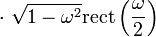
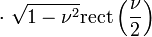
The following tables record some closed form Fourier transforms. For functions ƒ(x) , g(x) and h(x) denote their Fourier transforms by , , and  respectively. Only the three most common conventions are included.
[edit] Functional relationships
The Fourier transforms in this table may be found in (Erdélyi 1954) or the appendix of (Kammler 2000)
| Function | Fourier transform unitary, ordinary frequency |
Fourier transform unitary, angular frequency |
Fourier transform non-unitary, angular frequency |
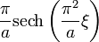
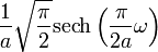
Remarks | |
|---|---|---|---|---|---|
 |

|
  |

|
||
| 101 |  |
 |
 |
 |
Linearity |
| 102 |  |
 |
 |
 |
Shift in time domain |
| 103 |  |
 |
 |
 |
Shift in frequency domain, dual of 102 |
| 104 |  |
 |
 |
 |
If  is large, then is concentrated around 0 and spreads out and flattens. is large, then is concentrated around 0 and spreads out and flattens. |
| 105 |  |
 |
 |
 |
Here needs to be calculated using the same method as Fourier transform column. Results from swapping "dummy" variables of  and and  . . |
| 106 |  |
 |
 |
 |
|
| 107 |  |
 |
 |
 |
This is the dual of 106 |
| 108 |  |
 |
 |
 |
The notation f * g denotes the convolution of f and g — this rule is the convolution theorem |
| 109 |  |
 |
 |
 |
This is the dual of 108 |
| 110 | For f(x) a purely real even function |  , and , and  are purely real even functions. are purely real even functions. |
|||
| 111 | For f(x) a purely real odd function | , and  are purely imaginary odd functions. are purely imaginary odd functions. |
|||

[edit] Square-integrable functions
The Fourier transforms in this table may be found in (Campbell & Foster 1948), (Erdélyi 1954), or the appendix of (Kammler 2000)
| Function | Fourier transform unitary, ordinary frequency |
Fourier transform unitary, angular frequency |
Fourier transform non-unitary, angular frequency |
Remarks | |
|---|---|---|---|---|---|
| f(x) |
|
|
|
||
| 201 |  |
 |
 |
 |
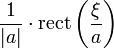
The rectangular pulse and the normalized sinc function, here defined as sinc(x) = sin(πx)/(πx) |
| 202 |  |
 |
 |
 |
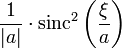
Dual of rule 201. The rectangular function is an ideal low-pass filter, and the sinc function is the non-causal impulse response of such a filter. |
| 203 |  |
 |
 |
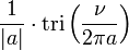 |
The function tri(x) is the triangular function |
| 204 |  |
 |
 |
 |
Dual of rule 203. |
| 205 |  |
 |
 |
 |
The function u(x) is the Heaviside unit step function and a>0. |
| 206 |  |
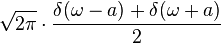
 |
 |
 |
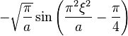
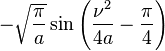
This shows that, for the unitary Fourier transforms, the Gaussian function exp(−αx2) is its own Fourier transform for some choice of α. For this to be integrable we must have Re(α)>0. |
| 207 |  |
 |
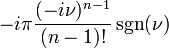
 |
 |
For a>0. |
| 208 |  |
 |
 |
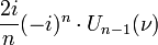 |
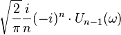
The functions Jn (x) are the n-th order Bessel functions of the first kind. The functions Un (x) are the Chebyshev polynomial of the second kind. See 315 and 316 below. |
| 209 |  |
 |
 |
 |
Hyperbolic secant is its own Fourier transform |

[edit] Distributions
The Fourier transforms in this table may be found in (Erdélyi 1954) or the appendix of (Kammler 2000)
| Function | Fourier transform unitary, ordinary frequency |
Fourier transform unitary, angular frequency |
Fourier transform non-unitary, angular frequency |
Remarks | |
|---|---|---|---|---|---|
| f(x) |
|
|
|
||
| 301 | 1 | δ(ξ) |  |
2πδ(ν) | The distribution δ(ξ) denotes the Dirac delta function. |
| 302 |  |
1 |  |
1 | Dual of rule 301. |
| 303 | eiax |  |
 |
2πδ(ν − a) | This follows from 103 and 301. |
| 304 | cos(ax) | 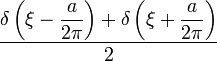 |
 |
 |
This follows from rules 101 and 303 using Euler's formula:  |
| 305 | sin(ax) |  |
 |
 |
This follows from 101 and 303 using  |
| 306 | cos(ax2) |  |
 |
 |
|
| 307 |  |
 |
 |
 |
|
| 308 |  |
 |
 |
 |
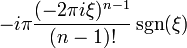
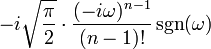
Here, n is a natural number and  is the n-th distribution derivative of the Dirac delta function. This rule follows from rules 107 and 301. Combining this rule with 101, we can transform all polynomials. is the n-th distribution derivative of the Dirac delta function. This rule follows from rules 107 and 301. Combining this rule with 101, we can transform all polynomials. |
| 309 |  |
− iπsgn(ξ) |  |
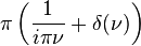
− iπsgn(ν) | Here sgn(ξ) is the sign function. Note that 1/x is not a distribution. It is necessary to use the Cauchy principal value when testing against Schwartz functions. This rule is useful in studying the Hilbert transform. |
| 310 |  |
 |
 |
 |
Generalization of rule 309. |
| 311 |  |
 |
 |
 |
|
| 312 | sgn(x) |  |
 |
 |
The dual of rule 309. This time the Fourier transforms need to be considered as Cauchy principal value. |
| 313 | u(x) |  |
 |
 |
The function u(x) is the Heaviside unit step function; this follows from rules 101, 301, and 312. |
| 314 | 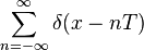 |
 |
 |
 |
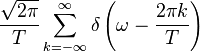
This function is known as the Dirac comb function. This result can be derived from 302 and 102, together with the fact that  as distributions. as distributions. |
| 315 | J0(x) | 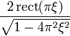 |
 |
 |
The function J0(x) is the zeroth order Bessel function of first kind. |
| 316 | Jn(x) |  |
 |
 |
This is a generalization of 315. The function Jn(x) is the n-th order Bessel function of first kind. The function Tn(x) is the Chebyshev polynomial of the first kind. |
[edit] Two-dimensional functions
| Function | Fourier transform unitary, ordinary frequency |
Fourier transform unitary, angular frequency |
Fourier transform non-unitary, angular frequency |
Remarks | |
|---|---|---|---|---|---|
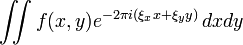
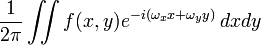
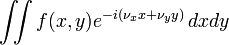
| f(x,y) | 
|

|

|
The variables ξx, ξy, ωx, ωy, νx and νy are real numbers. The integrals are taken over the entire plane. | |
| 401 | 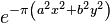 |
 |
 |
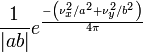 |
Both functions are Gaussians, which may not have unit volume. |
| 402 | 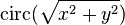 |
 |
 |
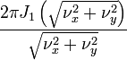 |
The function is defined by circ(r)=1 0≤r≤1, and is 0 otherwise. This is the Airy distribution and is expressed using J1 (the order 1 Bessel function of the first kind). (Stein & Weiss 1971, Thm. IV.3.3) |
[edit] Formulas for general n-dimensional functions
| Function | Fourier transform unitary, ordinary frequency |
Fourier transform unitary, angular frequency |
Fourier transform non-unitary, angular frequency |
Remarks | |
|---|---|---|---|---|---|
|
|
 |
|
||
| 501 | χ[0,1]( | x | )(1 − | x | 2)δ | π − δΓ(δ + 1) | ξ | − (n / 2) − δ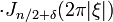 |
  |
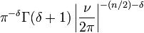  |
The function χ[0,1] is the characteristic function of the interval [0,1]. The function Γ(x) is the gamma function. The function Jn/2 + δ a Bessel function of the first kind with order n/2+δ. Taking n = 2 and δ = 0 produces 402. (Stein & Weiss 1971, Thm. 4.13) |

[edit] See also
[edit] References
|
|
This article includes a list of references or external links, but its sources remain unclear because it lacks inline citations. Please improve this article by introducing more precise citations where appropriate. (February 2008) |
- Bochner S.,Chandrasekharan K. (1949). Fourier Transforms. Princeton University Press.
- Bracewell, R. N. (2000), The Fourier Transform and Its Applications (3rd ed.), Boston: McGraw-Hill.
- Campbell, George; Foster, Ronald (1948), Fourier Integrals for Practical Applications, New York: D. Van Nostrand Company, Inc..
- Duoandikoetxea, Javier (2001), Fourier Analysis, American Mathematical Society, ISBN 0-8218-2172-5.
- Dym, H; McKean, H (1985), Fourier Series and Integrals, Academic Press, ISBN 978-0122264511.
- Erdélyi, Arthur, ed. (1954), Tables of Integral Transforms, 1, New Your: McGraw-Hill
- Grafakos, Loukas (2004), Classical and Modern Fourier Analysis, Prentice-Hall, ISBN 0-13-035399-X.
- Hörmander, L. (1976), Linear Partial Differential Operators, Volume 1, Springer-Verlag, ISBN 978-3540006626.
- James, J.F. (2002), A Student's Guide to Fourier Transforms (2nd ed.), New York: Cambridge University Press, ISBN 0-521-00428-4.
- Kaiser, Gerald (1994), A Friendly Guide to Wavelets, Birkhäuser, ISBN 0-8176-3711-7
- Kammler, David (2000), A First Course in Fourier Analysis, Prentice Hall, ISBN 0-13-578782-3
- Katznelson, Yitzhak (1976), An introduction to Harmonic Analysis, Dover, ISBN 0-486-63331-4
- Pinsky, Mark (2002), Introduction to Fourier Analysis and Wavelets, Brooks/Cole, ISBN 0-534-37660-6
- Polyanin, A. D.; Manzhirov, A. V. (1998), Handbook of Integral Equations, Boca Raton: CRC Press, ISBN 0-8493-2876-4.
- Rudin, Walter (1987), Real and Complex Analysis (Third ed.), Singapore: McGraw-Hill, ISBN 0-07-100276-6.
- Stein, Elias; Shakarchi, Rami (2003), Fourier Analysis: An introduction, Princeton University Press, ISBN 0-691-11384-X.
- Stein, Elias; Weiss, Guido (1971), Introduction to Fourier Analysis on Euclidean Spaces, Princeton, N.J.: Princeton University Press, ISBN 978-0-691-08078-9.
- Wilson, R. G. (1995), Fourier Series and Optical Transform Techniques in Contemporary Optics, New York: Wiley, ISBN 0471303577.
- Yosida, K. (1968), Functional Analysis, Springer-Verlag, ISBN 3-540-58654-7.
[edit] External links
- Fourier Series Applet (Tip: drag magnitude or phase dots up or down to change the wave form).
- Tables of Integral Transforms at EqWorld: The World of Mathematical Equations.
- Eric W. Weisstein, Fourier Transform at MathWorld.
- Fourier Transform Module by John H. Mathews
- The DFT “à Pied”: Mastering The Fourier Transform in One Day at The DSP Dimension

