Kelly criterion
From Wikipedia, the free encyclopedia
In probability theory, the Kelly criterion, or Kelly strategy or Kelly formula, or Kelly bet, is a formula used to determine the optimal size of a series of bets. In most gambling scenarios, and some investing scenarios under some simplifying assumptions, the Kelly strategy will do better than any essentially different strategy in the long run. It was described by J. L. Kelly, Jr, in a 1956 issue of the Bell System Technical Journal[1]. Edward O. Thorp demonstrated the practical use of the formula in a 1961 address to the American Mathematical Society[2] and later in his books Beat the Dealer[3] (for gambling) and Beat the Market[4] (with Sheen Kassouf, for investing).
Although the Kelly strategy's promise of doing better than any other strategy seems compelling, some economists have argued strenuously against it, mainly because an individual's specific investing constraints override the desire for optimal growth rate.[5] The conventional alternative is utility theory which says bets should be sized to maximize the expected utility of the outcome (to an individual with logarithmic utility, the Kelly bet maximizes utility, so there is no conflict). Even Kelly supporters usually argue for fractional Kelly (betting a fixed fraction of the amount recommended by Kelly) for a variety of practical reasons, such as wishing to reduce volatility, or protecting against non-deterministic errors in their advantage (edge) calculations.[6]
In recent years, Kelly has become a part of mainstream investment theory[7] and the claim has been made that well-known successful investors including Warren Buffett[8] and Bill Gross[9] use Kelly methods. William Poundstone wrote an extensive popular account of the history of Kelly betting in Fortune's Formula[5].
Contents |
[edit] Statement
For simple bets with two outcomes, one involving losing the entire amount bet, and the other involving winning the bet amount multiplied by the payoff odds, the Kelly bet is:
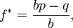
where
- f* is the fraction of the current bankroll to wager;
- b is the net odds received on the wager (that is, odds are usually quoted as "b to 1")
- p is the probability of winning;
- q is the probability of losing, which is 1 − p.
As an example, if a gamble has a 60% chance of winning (p = 0.60, q = 0.40), but the gambler receives 1-to-1 odds on a winning bet (b = 1), then the gambler should bet 20% of the bankroll at each opportunity (f* = 0.20), in order to maximize the long-run growth rate of the bankroll.
If the gambler has zero edge, i.e. if b = q/p, then the criterion will usually recommend the gambler bets nothing (although in more complex scenarios, where for instance a short priced favourite in a horse race may be worth covering to provide downside protection even though the only advantageous bet is on another outsider, will be correctly bet on to ensure the best compounding rate of return). If the edge is negative (b < q/p) the formula gives a negative result, indicating that the gambler should take the other side of the bet. For example, in standard American roulette, the bettor is offered an even money payoff (b = 1) on red, when there are 18 red numbers and 20 non-red numbers on the wheel (p = 18/38). The Kelly bet is -1/19, meaning the gambler should bet one-nineteenth of the bankroll that red will not come up. Unfortunately, the casino reserves this bet for itself, so a Kelly gambler will not bet.
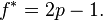
For even-money bets (i.e. when b = 1), the formula can be simplified to:

Since q = 1-p, this simplifies further to
[edit] Proof
For a rigorous and general proof, see Kelly's original paper[1] or some of the other references listed below. Some corrections can be found in: Optimal Gambling Systems For Favourable Games:- L. Breiman, University of California, Los Angeles.
We give the following non-rigorous argument for the case b = 1 to show the general idea and provide some insights.
When b = 1, the Kelly bettor bets 2p - 1 times initial wealth, W, as shown above. If she wins, she has 2pW. If she loses, she has 2(1 - p)W. Suppose she makes N bets like this, and wins K of them. The order of the wins and losses doesn't matter, she will have:

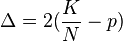
Suppose another bettor bets a different amount, (2p - 1 + Δ)W for some positive or negative Δ. He will have (2p + Δ)W after a win and [2(1 - p)- Δ]W after a loss. After the same wins and losses as the Kelly bettor, he will have:
![(2p+\Delta)^K[2(1-p)-\Delta]^{N-K}W \!](http://upload.wikimedia.org/math/a/4/b/a4b814d5ba30df6404506489e5905d33.png)
Take the derivative of this with respect to Δ and get:
![K(2p+\Delta)^{K-1}[2(1-p)-\Delta]^{N-K}W-(N-K)(2p+\Delta)^K[2(1-p)-\Delta]^{N-K-1}W\!](http://upload.wikimedia.org/math/1/2/f/12f40e12d0632addfa09de7b4509b3c7.png)
which equals zero if:
![K[2(1-p)-\Delta]=(N-K)(2p+\Delta) \!](http://upload.wikimedia.org/math/d/3/8/d386e009e6ba02a60a46a9d992e43c64.png)
which implies:
but:
so in the long run, final wealth is maximized by setting Δ to zero, which means following Kelly strategy.
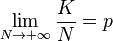
This illustrates that Kelly has both a deterministic and a stochastic component. If you knew K and N and had to pick a constant fraction of wealth to bet each time (otherwise you could cheat and, for example, bet zero after the Kth win knowing that the rest of the bets will lose), you will end up with the most money if you bet:
each time. This is true whether N is small or large. The "long run" part of Kelly is necessary because you don't know K in advance, just that as N gets large, K will approach pN. Someone who bets more than Kelly can do better if K > pN for a stretch, someone who bets less than Kelly can do better if K < pN for a stretch, but in the long run, Kelly always wins.
[edit] Reasons to bet less than Kelly
A natural assumption is that taking more risk increases the probability of both very good and very bad outcomes. One of the most important ideas in Kelly is that betting more than the Kelly amount decreases the probability of very good results, while still increasing the probability of very bad results. Since in reality we seldom know the precise probabilities and payoffs, and since overbetting is worse than underbetting, it makes sense to err on the side of caution and bet less than the Kelly amount.
Kelly assumes sequential bets that are independent (later work generalizes to bets that have sufficient independence). That may be a good model for some gambling games, but generally does not apply in investing and other forms of risk-taking. Suppose an investor is offered 10 different bets with 40% chance of winning and 2 to 1 payoffs (this is the example used above). Considering the bets one at a time, Kelly says to bet 10% of wealth on each, which means the investor's entire wealth is at risk. That risks ruin, especially if the payoffs of the bets are correlated.
The Kelly property appears "in the long run" (that is, it is an asymptotic property). To a person, it matters whether the property emerges over a small number or a large number of bets. It makes sense to consider not just the long run, but where losing a bet might leave you in the short and medium term as well. A related point is that Kelly assumes the only important thing is long-term wealth. Most people also care about about the path to get there. Two people dying with the same amount of money need not have had equally happy lives. Kelly betting leads to highly volatile short-term outcomes which many people find unpleasant, even if they believe they will do well in the end.
One of the most unrealistic assumptions in the Kelly derivation is that wealth is both the goal and the limit to what you can bet. Most people cannot bet their entire wealth, for example it is illegal to bet your future human capital (you cannot sell yourself into slavery). On the other hand, people can bet money they do not have by borrowing. A person who is allowed to bet more than his wealth might choose to bet more than Kelly (if you know you can always borrow a new stake, it makes sense to take more risk) while someone who is constrained to bet much less than his wealth (say a young college graduate with high lifetime potential earnings but no cash or credit) is forced to bet less.
[edit] Bernoulli
In a 1738 article, Daniel Bernoulli suggested that when you have a choice of bets or investments you should choose that with the highest geometric mean of outcomes. This is mathematically equivalent to the Kelly criterion, although the motivation is entirely different (Bernoulli wanted to resolve the St. Petersburg paradox). The Bernoulli article was not translated into English[10] until 1956 but the work was well-known among mathematicians and economists.
[edit] See also
[edit] Cited references
- ^ a b J. L. Kelly, Jr, A New Interpretation of Information Rate, Bell System Technical Journal, 35, (1956), 917–926
- ^ E. O. Thorp, Fortune's Formula: The Game of Blackjack, American Mathematical Society, January 1961
- ^ E. O. Thorp, Beat the dealer: a winning strategy for the game of twenty-one. A scientific analysis of the world-wide game known variously as blackjack, twenty-one, vingt-et-un, pontoon or Van John, Blaisdell Pub. Co (1962), ASIN: B0006AY2QW
- ^ Edward O. Thorp and Sheen T. Kassouf, Beat the Market: A Scientific Stock Market System, Random House (1967), ISBN: 978-0394424392
- ^ a b William Poundstone, Fortune's Formula: The Untold Story of the Scientific Betting System That Beat the Casinos and Wall Street, Hill and Wang, New York, 2005. ISBN 0809046377
- ^ E. O. Thorp, The Kelly Criterion: Part I, Wilmott Magazine, May 2008
- ^ S.A. Zenios and W.T. Ziemba, Handbook of Asset and Liability Management, North Holland (2006), ISBN: 978-0444508751
- ^ Mohnish Pabrai, The Dhandho Investor: The Low - Risk Value Method to High Returns, Wiley (2007), ISBN: 978-0470043899
- ^ E. O. Thorp, The Kelly Criterion: Part II, Wilmott Magazine, September 2008
- ^ Daniel Bernoulli, Exposition of a New Theory on the Measurement of Risk, Econometrica, 22(1), (english translation: 1956, original article:1738), 23–36
[edit] External links
- Original Kelly paper
- Bayesian Kelly Criterion
- Multi-variable Kelly Calculator for Sports Bettors
- Kelly Criterion by Tom Weideman
- Generalized Kelly Criterion For Multiple Outcomes and Financial Investors
- portfolio analyzer which maximizes expected log return (Kelly criterion) for one risk free bond and a group of risky alpha Levy stable assets
- Kelly staking plan calculator
- Daniel Bernoulli - Exposition of a New Theory on the Measurement of Risk, translated to english

